Kernel-bounded clustering for spatial transcriptomics enables scalable discovery of complex spatial domains

Abstract

Spatial transcriptomics are a collection of technologies that have enabled characterization of gene expression profiles and spatial information in tissue samples. Existing methods for clustering spatial transcriptomics data have primarily focused on data transformation techniques to represent the data suitably for subsequent clustering analysis, often using an existing clustering algorithm. These methods have limitations in handling complex data characteristics with varying densities, sizes, and shapes (in the transformed space on which clustering is performed), and they have high computational complexity, resulting in unsatisfactory clustering outcomes and slow execution time even with GPUs. Rather than focusing on data transformation techniques, we propose a new clustering algorithm called kernel-bounded clustering (KBC). It has two unique features: (1) It is the first clustering algorithm that employs a distributional kernel to recruit members of a cluster, enabling clusters of varying densities, sizes, and shapes to be discovered, and (2) it is a linear-time clustering algorithm that significantly enhances the speed of clustering analysis, enabling researchers to effectively handle large-scale spatial transcriptomics data sets. We show that (1) KBC works well with a simple data transformation technique called the Weisfeiler-Lehman scheme, and (2) a combination of KBC and the Weisfeiler-Lehman scheme produces good clustering outcomes, and it is faster and easier-to-use than many methods that employ existing clustering algorithms and data transformation techniques.

Figure 1.

The workflow of clustering analysis using KBC. (A) Beginning with a spatial transcriptomics (ST) data set, the spatial information L and the gene expression information E are integrated to produce a graph that contains both cell location and gene expression information. (B) A graph-embedding scheme converts a graph into a vector representation, as shown on the left, which is ready to be used for clustering. The illustration shows the two steps of the proposed KBC algorithm.

Figure 2.

First ablation study. Comparing different data transformation methods using the same k-means clustering. (A) The violin plots show the ARI and NMI results of all 12 slices of DLPFC. The runtimes are shown in a bar chart. (B) The detailed clustering results of different embedding methods together with the ground-truth labels are shown for the slice 151673. Here, SpatialPCA, WL, and PCA ran on CPU only. Other methods ran on GPU.

Figure 3.

Second ablation study. Comparing different clustering algorithms using the same SpatialPCA embedding. (A) The violin plots show the ARI and NMI results of all 12 slices of DLPFC of the seven clustering algorithms. The runtimes are showed in a bar chart. (B) The detailed clustering results of different clustering methods are shown for the slice 151673. Only SpaGCN ran on GPU; others ran on CPU.

Figure 4.

Examining the ability to find clusters of varied densities and overlapping clusters on two synthetic data sets: 3Gaussians and StripC. (A) The bar charts (in terms of ARI and NMI) of the five clustering methods on 3Gaussians. (B) The bar charts of the five clustering methods on StripC. (C) The ground truth and the clustering results of the five clustering methods on 3Gaussians. (D) The ground truth and the clustering results of the five clustering methods on StripC.

Figure 5.

Clustering outcomes on the density contour map created using multidimensional scaling (MDS) (Torgerson 1952). MDS reduces the number of dimensions of the features derived from SpatialPCA (identified to be the best data transformation method previously). The density is estimated using kernel density estimation (Scott 2015) on the space of the MDS reduced dimensions. The data transformation methods used are SpatialPCA, stLearn, and Stagate, and the clustering methods are as employed in their respective papers (Dong and Zhang 2022; Shang and Zhou 2022; Pham et al. 2023), except the proposed KBC.

Figure 6.

Scaleup test result for different clustering algorithms on the Slide-seq V2 mouse hippocampus data set (Stickels et al. 2021). This data set facilitates the creation of increasing larger subsets for the test. The data sizes range from 1000 to 160,000. We reduce the dimensionality of the data set using principal component analysis (PCA) and retain the top 20 principal components, which capture the majority of the variance in the data set. This is used for all algorithms. The data set size has 1000 points at data size ratio = 1. BayesSpace has no results on larger data sets because it took >48 h. Note that SpatialPCA and stLearn employ Walktrap and k-means/Louvain, respectively, as their clustering algorithms. Only SpaGCN's runtime is in GPU seconds. Note that the linear time has a gradient of one in the runtime ratio plot (shown by the line labeled as linear). Those runtimes that are worse than linear have a higher gradient.

Figure 7.

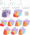
Application of KBC to the HER2 tumor data. (A,B) The violin plots of results obtained from different methods (for sections A1 to H1). (C) The boxplot in terms of local inverse Simpsons index (LISI) (Korsunsky et al. 2019) for different sections (from A1 to H1). A lower LISI value indicates a more uniform cluster of adjacent spatial domains. Thus, the smaller LISI the better. The red cross points are outliers of the LISI. (D) The histology image and manual annotation plot of section H1. (E) Clustering outcomes of four methods: KBC, BayesSpace (k-means), SpaGCN (Louvain), and SpatialPCA for section H1. The bottom row indicates three example cluster outcomes of BayesSpace and SpaGCN, but they employ the initial clusters produced by Mclust, k-means, and Louvain, respectively. Two results of SpaGCN use Louvain to produce the initial clusters but with different parameter settings.

Figure 8.

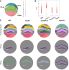
Application of KBC to the mouse hippocampus data. (A) Allen Brain Atlas P56 coronal. The diagram shows the structure of the mouse hippocampus. (B) The LISI index of the clustering results of KBC, SpaGCN, SpatialPCA, and Stagate. (C) A comparison of four clustering results on the CA1sp domain and the DG-sg domain.

Figure 9.

Application of KBC to the DLPFC data. (A,B) The violin plots of the results obtained from six different methods on the DLPFC data set. (C) The boxplot of clustering LISI of the six different methods on the DLPFC data set. (D) Histology image, manual annotation (Maynard et al. 2021), and the clustering results of KBC, BayesSpace, SpaGCN, SpatialPCA, Stagate, and stLearn plotted on DLPFC slice 151669.

Figure 10.

Results of the further ablation studies on four clustering methods and two data transformation methods using the HVG and SVG simulated data sets.

References

1. Aggarwal CC. 2015. Data mining: the textbook, Vol. 1. Springer, Cham, Switzerland.
1. Andersson A, Larsson L, Stenbeck L, Salmén F, Ehinger A, Wu SZ, Al-Eryani G, Roden D, Swarbrick A, Borg Å, et al. 2021. Spatial deconvolution of HER2-positive breast cancer delineates tumor-associated cell type interactions. Nat Commun 12: 6012. 10.1038/s41467-021-26271-2 - DOI - PMC - PubMed
1. Arthur D, Vassilvitskii S. 2006. How slow is the k-means method? In SCG '06: Proceedings of the twenty-second annual symposium on Computational Geometry, Sedona, AZ, pp. 144–153. 10.1145/1137856.1137880 - DOI
1. Asp M, Bergenstråhle J, Lundeberg J. 2020. Spatially resolved transcriptomes: next generation tools for tissue exploration. Bioessays 42: 1900221. 10.1002/bies.201900221 - DOI - PubMed
1. Bandaragoda TR, Ting KM, Albrecht D, Liu FT, Zhu Y, Wells JR. 2018. Isolation-based anomaly detection using nearest-neighbor ensembles. Comput Intell 34: 968–998. 10.1111/coin.12156 - DOI
LinkOut - more resources