Community estimate of global glacier mass changes from 2000 to 2023

Abstract

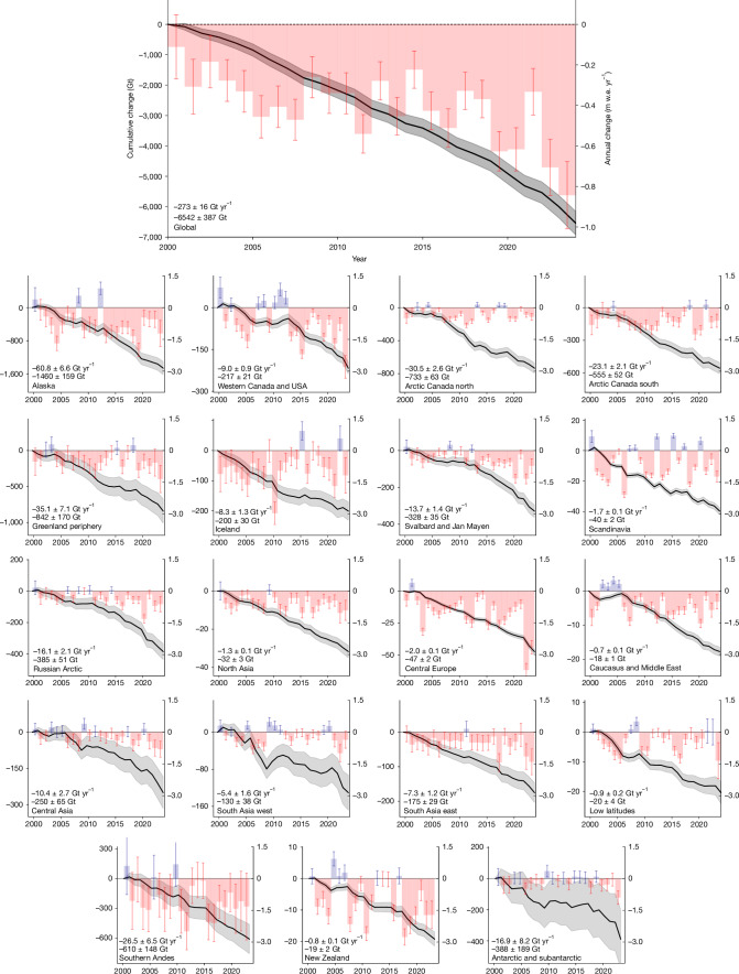
Glaciers are indicators of ongoing anthropogenic climate change¹. Their melting leads to increased local geohazards², and impacts marine³ and terrestrial^4,5 ecosystems, regional freshwater resources⁶, and both global water and energy cycles^7,8. Together with the Greenland and Antarctic ice sheets, glaciers are essential drivers of present^9,10 and future^11-13 sea-level rise. Previous assessments of global glacier mass changes have been hampered by spatial and temporal limitations and the heterogeneity of existing data series^14-16. Here we show in an intercomparison exercise that glaciers worldwide lost 273 ± 16 gigatonnes in mass annually from 2000 to 2023, with an increase of 36 ± 10% from the first (2000-2011) to the second (2012-2023) half of the period. Since 2000, glaciers have lost between 2% and 39% of their ice regionally and about 5% globally. Glacier mass loss is about 18% larger than the loss from the Greenland Ice Sheet and more than twice that from the Antarctic Ice Sheet¹⁷. Our results arise from a scientific community effort to collect, homogenize, combine and analyse glacier mass changes from in situ and remote-sensing observations. Although our estimates are in agreement with findings from previous assessments^14-16 at a global scale, we found some large regional deviations owing to systematic differences among observation methods. Our results provide a refined baseline for better understanding observational differences and for calibrating model ensembles^12,16,18, which will help to narrow projection uncertainty for the twenty-first century^11,12,18.

Fig. 1. Global glacier mass changes from 2000 to 2023.

Regional and global glacier mass changes from 2000 to 2023 as percentage loss (red slice in the pie chart) based on the glacier mass in 2000 (size of the pie chart). The coloured stripes under each pie chart represent annual specific mass changes (in metre water equivalent) for our combined estimate (indicated with an asterisk) together with combined results from DEM differencing and glaciological observations (Dg), altimetry (A) and gravimetry (G). Regional results are represented for hydrological years, that is, running from 1 October to 30 September in the Northern Hemisphere, 1 April to 31 March in the Southern Hemisphere and over the calendar year in the low latitudes. Global results are aggregated for calendar years. Source Data

Fig. 2. Annual and cumulative glacier mass change from 2000 to 2023.

Cumulative and annual glacier mass changes since 2000 for the 19 glacier regions (hydrological years) and aggregated to global sums (calendar years). Cumulative mass changes (left y axis, Gt) are shown as black curves, with values for mean annual change rate (Gt yr⁻¹) and cumulative change (Gt) for the entire period given in the bottom left corner. Annual mass changes (right y axis, m w.e. yr⁻¹) are coloured in blue and red for years with positive and negative mass changes, respectively. Uncertainties are given as 95% confidence intervals. It is noted that the left y axis differs for each subplot whereas the right y axis is the same for all regions. Source Data

Extended Data Fig. 1. Data submissions to the intercomparison exercise.

The figure provides an overview of research teams (left, in alphabetic order) participating in GlaMBIE with their selection of sensors or products (middle left) used for computing glacier mass-change estimates from different observation methods (middle right) for the 19 regions (right). From the 233 regional results, 195 (coloured lines) were used to compute our combined estimates, and 38 (grey lines) were excluded based on regional confidence levels of observation methods (see Methods). Colours follow observation methods. A more detailed overview of all data contributions is given in Supplementary Information Tables 1 and 2. The figure was produced with SankeyMATIC. Source Data

Extended Data Fig. 2. Principal approach and workflow of the intercomparison exercise.

The schematic diagram illustrates the principal approach (a) to combine input data from different observational sources. After selection and homogenization, each dataset is separated into its annual variability (β) and long-term trend $\left(\overline{B}\right)$ by de-trending. The annual variabilities from multiple input data are averaged to one time series and added to each long-term trend. The new set of re-trended time series are averaged to one combined estimate. In the GlaMBIE workflow (b), this approach is applied to combine (i) the annual variability from glaciological observations with long-term trends from DEM differencing, (ii) multiple input data from altimetry, (iii) multiple input data from gravimetry, and finally to (iv) combine these three results among the different observation methods. Finally, the region estimates are corrected from hydrological to calendar years and for regional area changes and cumulated to a global estimate. More details on the approach are provided in the Methods.

Extended Data Fig. 3. Regional mass-change rates per observation method.

For each region (rows), mean specific mass-change rates (shown as markers) and interannual variability (one standard deviation, shown as lines) are compared among different methods over common observation periods for altimetry (left column) and gravimetry (right column). The common observation periods are shown as decimal years (bottom right). The gravimetry period does not include the hydrological year 2007/08. The combined estimates include only the observation methods indicated by complete markers and solid lines. Empty markers or dashed lines indicate results not considered for the combined estimates. Differences between observation methods and related uncertainties are given in Extended Data Table 2. Source Data

Extended Data Fig. 4. Glacier mass-change estimates in comparison with IPCC results.

Comparison of our combined annual glacier mass changes (in Gt) with mean annual mass-change rates (in Gt yr⁻¹) from past IPCC reports^,, for regional aggregations at the global level (a), for Greenland and Antarctic periphery (c), regions with a large glacier area (e, excluding c), and regions with a small glacier area (g). The subplots on the right (b, d, f, h) show mean annual mass-change rates over the three IPCC assessment periods (AR5: 2003–2009, SROCC: 2006–2015, AR6: 2000–2019), and the GlaMBIE period (2000–2023). For the latter, we show our combined estimates (black line with grey error bars) together with the change rates from glaciological observations, DEM differencing, altimetry, and gravimetry, if available. We note that the long-term trends from glaciological observations and gravimetry in regions with a small glacier area were not used for the combined estimates. Uncertainties are shown for 95% confidence intervals. Source Data

Extended Data Fig. 5. Glacier mass-change observations and model projections.

Comparison of observed cumulative glacier mass changes (in Gt, left y-axis) and corresponding cumulative sea-level equivalents (in mm, right y-axis) since 2000 with ensemble projections for 2007–2040 and 2040–2100 from the glacier model intercomparison project (GlacierMIP2, based on CMIP5), as used in IPCC AR6 (a) and from a more recent model study (based on CMIP6) (b). Glacier mass-change observations (black line) are accompanied by their 95% confidence intervals (grey shading). For the projections, ensemble medians (blue and red lines) are shown with 90 percentile ranges (blue and red shadings) for low and high emission scenarios, respectively. Projections have been offset at their start date (2007) to fit the cumulative value of the observations. Regional comparisons are shown in Supplementary Information Figs. 20 and 21. Source Data

References

1. Bojinski, S. et al. The concept of essential climate variables in support of climate research, applications, and policy. Bull. Am. Meteorol. Soc.95, 1431–1443 (2014).
1. Haeberli, W. & Whiteman, C. in Snow and Ice-Related Hazards, Risks, and Disasters (eds Shroder, J. F. et al.) 1–34 (Elsevier, 2015); 10.1016/B978-0-12-394849-6.00001-9.
1. Hopwood, M. J. et al. How does glacier discharge affect marine biogeochemistry and primary production in the Arctic? Cryosphere14, 1347–1383 (2020).
1. Ficetola, G. F. et al. The development of terrestrial ecosystems emerging after glacier retreat. Nature632, 336–342 (2024). - PubMed
1. Bosson, J. B. et al. Future emergence of new ecosystems caused by glacial retreat. Nature620, 562–569 (2023). - PubMed
Publication types