Multi-tissue transcriptomic aging atlas reveals predictive aging biomarkers in the killifish

Abstract

Aging is associated with progressive tissue dysfunction, leading to frailty and mortality. Characterizing aging features, such as changes in gene expression and dynamics, shared across tissues or specific to each tissue, is crucial for understanding systemic and local factors contributing to the aging process. We performed RNA-sequencing on 13 tissues at 6 different ages in the African turquoise killifish, the shortest-lived vertebrate that can be raised in captivity. This comprehensive, sex-balanced 'atlas' dataset reveals the varying strength of sex-age interactions across killifish tissues and identifies age-altered biological pathways that are evolutionarily conserved. Demonstrating the utility of this resource, we discovered that the killifish head kidney exhibits a myeloid bias during aging, a phenomenon more pronounced in females than in males. In addition, we developed tissue-specific 'transcriptomic clocks' and identified biomarkers predictive of chronological age. We show the importance of sex-specific clocks for selected tissues and use the tissue clocks to evaluate a dietary intervention in the killifish. Our work provides a comprehensive resource for studying aging dynamics across tissues in the killifish, a powerful vertebrate aging model.

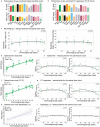
Extended Data Figure 1:. Metadata for the multi-tissue killifish transcriptomic aging atlas

(a) Kaplan-Meier survival curves for the two cohorts (left, middle) from which samples for RNA-sequencing were derived (left, 19 females, 24 males; middle, 31 females, 33 males). On the right is the survival curve for both cohorts combined (50 females, 57 males). Blue, male survival curve; red, female survival curve. Yellow and additional ticks on x-axis, sample collection windows. F, female; M, male. (b) Number of samples analyzed for each tissue, sex, and age group in this study. The red numbers denote incidences of sample dropout. ‘—’ indicates ‘not applicable.’ (C) Bar plots of the median percent variance explained across all genes expressed in an tissue for the covariates of age (left), sex (middle), and the interaction term sex:age (right).

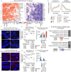
Extended Data Figure 2:. Cross-tissue pathways enriched for the genes correlated with age.

Male (M) vs. female (F) gene set enrichment analysis (GSEA) results, identifying the shared or unique pathways enriched for the genes upregulated or downregulated with age in the 13 tissues. For females and males, separately, tissues are clustered by similarity of enrichment as calculated by the product of the NES and −log(FDR). NES, normalized enrichment score. Dot size, −log10 of the adjusted p-value (i.e., false discovery rate [FDR] after multiple hypotheses testing).

Extended Data Figure 3:. Sex-specific pathways enriched for the genes correlated with age.

Male (M) vs. female (F) gene set enrichment analysis (GSEA) results in the 13 tissues, identifying the GO terms showing opposite signs of upregulation or downregulation with age in the two sexes, and those for which the change with age is significantly in only one sex (‘sex-divergent’). NES, normalized enrichment score. Dot size, −log10 of the adjusted p-value (i.e., false discovery rate [FDR] after multiple hypotheses testing). Boxes indicate the main sex-divergent GO terms in each tissue.

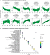
Extended Data Figure 4:. Tissue-specific gene expression dynamics for the gut and muscle

(a) Hierarchical clustering of the gene expression trajectories for the gut (sex-combined), highlighting cluster 8. The average trajectory for the cluster is depicted by the black line. The most highly significant GO term from Hypergeometric GO enrichment (terms related to Biological Processes) is listed, as well as the number of genes making up the cluster. (b) Hypergeometric GO enrichment (terms related to Biological Processes) for the genes in gut cluster 8. Select significantly enriched (adjusted p-value < 0.05) GO terms for each cluster are plotted. Dot color represents the enrichment score of each GO term, with the maximum value of the scale adjusted to 15 to improve color resolution of GO terms with lower enrichment. Dot size, −log10 of the adjusted p-value (i.e., false discovery rate [FDR] after multiple hypotheses testing). (c) Hierarchical clustering of the gene expression trajectories for the muscle (sex-combined), highlighting cluster 7. The average trajectory for the cluster is depicted by the black line. As in panel a, the most highly significant GO term from hypergeometric GO enrichment is listed, as well as the number of genes making up the cluster. (d) Hypergeometric GO enrichment for muscle cluster 7, analysis conducted as in panel b.

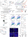
Extended Data Figure 5:. The aging killifish kidney marrow changes in gene expression and cell-type composition.

(a) Dot plot of gene expression for genes in Fig. 4b, showing cell-type specific enrichment. Dot color indicates the level of expression, and dot size indicates the percentage of cells expressing the gene. (b) Flow cytometry gating scheme, showing representative gating workflow from raw event data to live cells. (c) Principal Component (PC) Analysis of the dissociated male head kidney cell populations that were FACS-sorted based on the gating strategy as in panel b. Each dot is an individual animal (myeloid population: 3 fish; lymphoid population: 2 fish). These males were harvested from different ages (67, 88, and 201 days) to test whether the gating strategy can be applied to different age groups. (d) Heatmap showing the expression of myeloid and lymphoid cell type-specific markers (see panel a), clustered by samples. The expression of each gene is plotted as Z-scaled, DESeq2-normalized counts. (e) Scatterplot of the counts normalized by DESeq2 for irf4b (killifish gene name: irf4) in the head kidney transcriptome of the atlas dataset. Each dot is the expression of irf4b in an individual sample. Red, female (F). Blue, male (M). (f) UMAP (uniform manifold approximation and projection) plots of data from a killifish single-cell RNA-sequencing tissue atlas, with overlayed expression levels for irf4a (left) and irf4b (right). (g) Co-expression UMAP showing the expression level of irf4a and ptprc. Data were derived from the tissue atlas. The irf4a^high ptprc^low cells are red (1368 cells in the source dataset), irf4a^low ptprc^high cells are blue (11,635 cells), and irf4a^high ptprc^high cells are purple (904 cells). (h) Example single-z-plane HCR image of young male head kidney tissue, with cross section of renal tubule epithelium encircled by white dashed lines. Outside of these white dashed boundaries is the interstitial space, where hematopoietic tissue resides. Quantification of the irf4a transcripts was performed for the interstitial space. Scale bar, 10 μm.

Extended Data Figure 6:. BayesAge 2.0 leads to less overfitting than Elastic Net and Principal Component regression models.

(a-b) Bar plots of the performance metrics for (a) Elastic Net regression tissue clocks and (b) Principal Component regression tissue clocks, using the coefficient of determination (R²) for the relationship between chronological and predicted age and the mean absolute error (MAE). (c) Residual plots for the optimal brain clock modeled with BayesAge 2.0. Left, using difference between predicted transcriptomic age (tAge) and the line of best fit. Right, difference between predicted transcriptomic age (tAge) and chronological age. The ‘optimal’ BayesAge clock for a tissue is defined as the clock with the most concordance between chronological and predicted age. (d) Scatterplot of the tissue transcriptomic age (tAge) vs. chronological age for measuring the prediction accuracy of the optimal brain sex-combined tissue clock using Elastic Net regression. The coefficient of determination (R²) for the relationship between chronological and predicted age and the mean absolute error (MAE) are listed in graphs. The ‘optimal’ Elastic Net tissue clock is defined as the clock with the optimal combination of α and λ such that model error is minimized. (e) Residual plots for the optimal brain Elastic Net regression clock, calculated and plotted as in panel c. (f) Scatterplot of age predictions versus chronological age as in panel d for the optimal brain Principal Component regression (PC-R) clock. The ‘optimal’ PC-R tissue clock is defined as the clock with the optimal number of principal components such that there is the most concordance between chronological and predicted age. (g) Residual plots for the optimal brain PC-R clock calculated and plotted as in panels c and e. (h) Scatterplot of age predictions versus chronological age for the optimal ovary clock, the lowest performing tissue clock using BayesAge 2.0. (i) Residual plots for the optimal ovary BayesAge 2.0 clock, calculated and plotted as in panels c, e, and g.

Extended Data Figure 7:. The brain and testis transcriptomic aging clocks are among the highest performing BayesAge 2.0 clocks across killifish tissues.

(a) Scatterplot of the tissue transcriptomic age (tAge) vs. chronological age for measuring the prediction accuracy of the optimal brain sex-combined tissue clock, which is the model that corresponds to the most concordance between chronological and predicted age among all the gene number tested. The coefficient of determination (R²) between chronological and predicted age, as well as the mean absolute error (MAE), is listed in graphs. (b) The gene frequency scatterplots of the top 10 overall age-correlated genes trained on the sex-combined brain samples are shown. The black line is the locally weighted scatterplot smoothing (LOWESS) regression fit across time. (c, d) The scatterplots of tAge vs. chronological age (c) and gene frequency (d) were generated as in panels a and b, but for the testis.

Extended Data Figure 8:. The sex-specific liver transcriptomic aging clocks predict dietary restriction results in ‘younger’ ages.

(a, b) The predicted tAge difference between the ad libitum (AL) or dietary-restricted (DR) conditions observed across a range of clock gene numbers used for the male (panel a) or female (panel b) liver clocks. F, female; M, male. The median (orange) or mean (blue) predicted tAge was calculated from the 4 animals for each condition (AL or DR), and then the prediction difference in tAge was calculated by subtracting the median or mean in DR from that of the AL condition. Dotted line, AL and DR have the same predicted tAge. Below the dotted line indicates the DR condition is predicted to be ‘younger’ than the AL condition. The transcriptomic data were derived from a published dataset. (c) Predicted tAges for the AL and DR conditions, male only, with each dot representing the predicted tAge of individual fish (4 fish per condition) when a specific clock gene number was used in the model. The box plots include the median, 25 (Q1), 75 (Q3) percentiles, and the whiskers include Q3+1.5×(Q3-Q1) and Q1−1.5×(Q3-Q1). At each gene number used for the model, Mann-Whitney test was used to test the significance of difference between the AL and DR conditions. (d) Predicted tAges for the AL and DR conditions, female only, plotted as described in panel c.

Figure 1:. A multi-tissue killifish transcriptomic aging atlas reveals shared and tissue-specific of age effect on different tissues

(a) Schematic for the killifish transcriptomic aging atlas. Thirteen tissues from males and females were collected for RNA-sequencing at the indicated timepoints (the animal numbers sampled are listed) from two independent cohorts of the GRZ killifish strain. (b) Principal component analysis (PCA) for the 677 samples reveals clear clustering by tissue identity. Symbol shape, biological sex (F, female; M, male). Symbol color, tissue type. (c) Tissues have varying numbers of age-correlated genes, as shown by the Spearman’s rank correlation (ρ) distribution for all the post-filtered genes in each tissue. Each dot is one gene. Male and female samples are analyzed together for each tissue and time point in panels c to e. (d) Each tissue has distinct proportion of age-correlated genes in its transcriptome. Upregulated with age, Spearman’s rank correlation ρ > 0.5. Downregulated with age, ρ < −0.5. (e) Proportion of differentially expressed genes between males and females (sex-dimorphic genes) for each tissue, at each binned age level. A break in the y-axis is denoted by double slashed lines. (f) Male (M) vs. female (F) gene set enrichment analysis (GSEA) results, identifying the pathways significantly enriched for the genes upregulated or downregulated with age in each tissue. NES, normalized enrichment score. Dot size, −log10 of the adjusted p-value (i.e., false discovery rate [FDR] after multiple hypotheses testing). (g) Heatmap of select GO terms, plotting the male and female Spearman’s rank correlations of the genes that drive each GO term.

Figure 2:. Cross-tissue comparison reveals shared age-correlated genes and pathways.

(a) Spearman’s rank correlation (ρ) heatmaps for the genes upregulated (left) or downregulated (right) with age shared across at least 6 tissues. Gray box, Spearman’s correlation was not calculated because the expression level of a particular gene was lower than the expression threshold (TPM > 0.5 in >80% of samples). Killifish gene names are shown as lowercase letters, and additional protein-coding killifish genes are annotated using the human ortholog gene names (uppercase). The genes named after gene loci numbers (e.g., LOC107378024) lack human orthologs. (b) Z-scaled locally estimated scatterplot smoothing (LOESS) regression fits of the gene expression trajectories across age for the genes ncRNA-3777 and IGF2BP3. (c, d) Representative maximum z-projected HCR (RNA in situ) images for ncRNA-3777 and IGF2BP3 mRNAs in male and female guts, at young (57–60 days) and old (120–130 days) ages. Scale bar, 5 μm. F, female; M, male. (e) Quantification of HCR images as the average number of ncRNA-3777 transcripts per cell. Each dot is an animal, and four animals are analyzed for each condition. In-graph statistics, Mann-Whitney test. Below-graph statistics, two-way ANOVA with age, sex, and age-sex interaction as variables. (f) Normalized RNA-seq counts for the ncRNA-3777 gene in the male and female guts across binned age groups. (g, h) Quantification and statistics were performed as in panels e and f, respectively, for IGF2BP3. Four animals are analyzed for each condition. (i) Hypergeometric GO enrichment results for the genes upregulated (top) or downregulated (bottom) with age that are shared across at least 5 tissues. Dot size, −log10 of the adjusted p-value (i.e., false discovery rate [FDR] after multiple hypotheses testing).

Figure 3:. Tissue-specific gene expression dynamics for the brain

(a) Hierarchical clustering of the gene expression trajectories for the brain. Hierarchical clustering was performed on the locally estimated scatterplot smoothing (LOESS) regression aging trajectory of the gene expression in the brain for the 10,847 genes expressed in all tissues, resulting in 10 clusters of gene expression behavior over time. The average trajectory for the cluster is depicted by the black line. The most significant GO term from Hypergeometric GO enrichment (terms related to Biological Processes) for each cluster is listed. (b) Hypergeometric GO enrichment (terms related to Biological Processes) for the genes in each cluster. Select significantly enriched (adjusted p-value < 0.05) GO terms for each cluster are plotted. Dot color represents the enrichment score of each GO term, with the maximum value of the scale adjusted to 20 to improve color resolution of GO terms with lower enrichment. Dot size, −log10 of the adjusted p-value (i.e., false discovery rate [FDR] after multiple hypotheses testing). Clusters 10 does not have any significant GO terms, so the lowest p-value terms are plotted.

Figure 4:. The aging killifish kidney marrow changes in gene expression and cell-type composition.

(a) Principal Component (PC) Analysis of all head kidney transcriptomes coded by age (in days) and sex (female, F; male, M). (b) Dot plot of the select cell-type marker genes for lymphoid and myeloid lineage cells. If a gene is named after a gene locus number (e.g., ‘LOC107384571’), either the zebrafish homolog (all lowercase) or human homolog (all uppercase) is also written. The dot size is the −log10 of the adjusted p-value, and the dot color corresponds to the Spearman’s rank correlation ρ value calculated separately for each sex. The cell-type specificity of each gene’s expression was based on a published killifish kidney single-cell RNA-seq dataset (see Extended Data Fig. 5). (c) Hypergeometric GO enrichment (terms related to Biological Processes) for the genes upregulated (right) or downregulated (left) with age identified for the head kidney when both sexes were analyzed together. Dot color represents the enrichment score of each GO term. Dot size, −log10 of the adjusted p-value (i.e., false discovery rate [FDR] after multiple hypotheses testing). (d) Schematic of the flow cytometry assay to quantify different immune cell lineages in the killifish. Dissected head kidney tissue was dissociated into a single-cell suspension and analyzed by Fluorescence Activated Cell Sorting (FACS). (e) Representative forward-scatter vs side-scatter flow cytometry plots from male and female killifish. Myeloid and lymphoid gates are depicted as the percentage of total live cells. (f) Quantification of myeloid: lymphoid ratio (total myeloid events: total lymphoid events) from flow cytometry data. Each dot is an animal, and 12 males and 6–8 females at each time point were analyzed for panels e and f. Significance determined by Mann-Whitney test. (g) Scatterplot of the counts normalized by DESeq2 for irf4a (LOC107383908), with each dot representing the expression of irf4a in an individual sample in the atlas dataset. Red, female (F). Blue, male (M). (h) Representative maximum z-projected HCR images of male (top) and female (bottom) kidney sections at young or old ages. The sections were stained with DAPI (blue) and the HCR probes against irf4a (red) and ptprc (white) mRNAs. Scale bars, 5 μm. (i) Quantification of the HCR images in panel h. The average number of irf4a mRNAs per cell is plotted (only the interstitial regions were quantified). Each dot is an animal (4 animal per each sex and age group were quantified). In-graph statistics, Mann-Whitney test. Below-graph statistics, two-way ANOVA with age, sex, and age-sex interaction as variables.

Figure 5:. Tissue-specific transcriptomic aging clocks predicts tissue biological ages in aging and interventions.

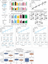
(a) Workflow of BayesAge 2.0, a Bayesian and locally weighted scatterplot smoothing (LOWESS) regression model behind the aging clocks. To train a tissue clock, Leave One Sample Out Cross-Validation (LOSO-CV) was used to generate testing-training splits of the data. In each iteration of LOSO-CV, one sample was used as a test set, while the rest of the tissue samples were used for training. This was performed k times, where k is the number of tissue samples available. Each time LOSO-CV was performed, a set of top age-associated genes (the highest absolute Spearman’s rank correlation values) was selected for the feature set. Then, the probability that the sample in the test set was a given age was calculated from the probability of the observed expression value for each selected gene in the sample at that age, assuming a Poisson distribution. The product of each gene-wise probability was computed to determine the age probability. The result was an age-probability distribution from which the age prediction was the highest probability age in this distribution. (b) Bar plots of the performance metrics for the BayesAge sex-combined tissue clocks, using the coefficient of determination (R²) for the relationship between chronological and predicted age and the mean absolute error (MAE). (c) Scatterplot of gut clock chronological age vs. the ‘transcriptomic age’ (tAge) for measuring the prediction accuracy of the highest performing gut sex-combined tissue clock. The ‘optimal’ BayesAge clock is defined as the model with the most concordance between chronological and predicted age among all the gene number tested. Bottom, the gene frequency scatterplots of the top 10 overall age-correlated genes trained on the sex-combined gut samples are shown. The pink line is the locally estimated scatterplot smoothing (LOESS) regression fit across time. (d) Bar plots of R² and MAE values for select clocks trained on sex-combined data (left, ‘S-C’), female data (middle, ‘F’), and male data (right, ‘M’). Selected tissues include highly transcriptionally sex-dimorphic tissues (gonad, kidney, liver), moderately transcriptionally sex-dimorphic tissues (gut, skin), and one weakly sex-dimorphic tissue (brain). (e) Accuracy of tAge predictions for the optimal sex-combined (left), male-only (middle), and female-only liver clocks (right). (f) Predicted ages for liver samples from male and female killifish fed on ad libitum (AL) or dietary restricted (DR) diets using sex-dimorphic liver clocks (data from a published dataset). Age prediction was performed using three different modeling strategies, BayesAge 2.0 (left), Elastic Net regression (middle), and Principal Component regression (right). Each dot in each box plot represents the predicted tAge for the liver transcriptome of an individual fish (4 fish per condition) and the gene set size or number of principal components used for age prediction is listed. For each model, Mann-Whitney test was used to test the significance of difference between the AL and DR conditions.

References

1. Lopez-Otin C., Blasco M. A., Partridge L., Serrano M. & Kroemer G. Hallmarks of aging: An expanding universe. Cell 186, 243–278, doi:10.1016/j.cell.2022.11.001 (2023). - DOI - PubMed
1. Yousefzadeh M. J. et al. Tissue specificity of senescent cell accumulation during physiologic and accelerated aging of mice. Aging Cell 19, e13094, doi:10.1111/acel.13094 (2020). - DOI - PMC - PubMed
1. Jin J., Yang X., Gong H. & Li X. Time- and Gender-Dependent Alterations in Mice during the Aging Process. Int J Mol Sci 24, doi:10.3390/ijms241612790 (2023). - DOI - PMC - PubMed
1. Hagg S. & Jylhava J. Sex differences in biological aging with a focus on human studies. Elife 10, doi:10.7554/eLife.63425 (2021). - DOI - PMC - PubMed
1. Serre-Miranda C. et al. Age-Related Sexual Dimorphism on the Longitudinal Progression of Blood Immune Cells in BALB/cByJ Mice. J Gerontol A Biol Sci Med Sci 77, 883–891, doi:10.1093/gerona/glab330 (2022). - DOI - PMC - PubMed
Publication types
LinkOut - more resources