Emergent patterns of patchiness differ between physical and planktonic properties in the ocean

Abstract

While a rich history of patchiness research has explored spatial structure in the ocean, there is no consensus over the controls on biological patchiness and how physical-ecological-biogeochemical processes and patchiness relate. The prevailing thought is that physics structures biology, but this has not been tested at basin scale with consistent in situ measurements. Here we use the slope of the relationship between variance vs spatial scale to quantify patchiness and ~650,000 nearly continuous (dx ~ 200 m) measurements - representing the Atlantic, Pacific, and Southern Oceans - and find that patchiness of biological parameters and physical parameters are uncorrelated. We show variance slope is an emergent property with unique patterns in biogeochemical properties distinct from physical tracers, yet correlated with other biological tracers. These results provide context for decades of observations with different interpretations, suggest the use of spatial tests of biogeochemical model parameterizations, and open the way for studies into processes regulating the observed patterns.

Fig. 1. The spatial extent and statistical distribution of the data used in this study.

Maps show the geographic distribution of chlorophyll-a (chla, a) and sea surface temperature (temp, b). The data includes 661,552 minute binned measurements. Insets show the histograms of both variables. The four numbers in panel (a) correspond to the example data shown in Fig. 2.

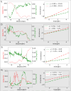
Fig. 2. Chlorophyll-a (chla) and temperature (temp) from four different transects and the resulting cascades of variance.

Examples of chla (green, solid) and temp (red, dashed) values along a leg (left panel in each pair) and the scale-dependent variance used to calculate the variance slope (Γ) derived from these legs (right panel in each pair). The variance slope can be seen in the legend for each panel on the right. The intercept indicated in each caption is a product of both the total amount of variance and the variance slope. The numbers of each panel (1–4) correspond to the locations in Fig. 1a.

Fig. 3. Geographic distributions of variance slope (Γ).

Maps show the Γ of chlorophyll-a (Γ_chla, a) and temperature (Γ_temperature, b). Insets in both panels show the histograms for these variables.

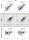
Fig. 4. Variance slope (Γ) comparisons between biogeochemical, physical, and biogeochemical vs physical variables.

Γ_chla correlates with the Γ of other biogeochemical parameters such as particulate attenuation (Γ_cp(443), a) and mean particle size (Γ_γ, b)_, and Γ_temperature correlates with the Γ of other physical parameters such as salinity (Γ_salinity, c) and (Γ_density, d), yet the Γ of biogeochemical vs physical variables don’t have a notable correlation (e, f). Larger colored markers correspond with the Longhurst provinces from Fig. 5. Contours partition the data’s probability mass function into five equal levels. N.b. correlations are shown for all data, not the Longhurst province means, and all plots have a p-value < 0.001.

Fig. 5. Longhurst provinces with S/V Tara legs overlaid in black.

Longhurst provinces that contain N = > 25 legs are shown geographically along with the S/V Tara legs within each province.

Fig. 6. Absolute value vs variance slope (Γ) for the variables under analysis.

The top rows (a–c) represent the biogeochemical variables: chlorophyll-a (chla), particulate attenuation at 443 nm (c_p(443)), and mean particle size (γ) and the and bottom rows (d–f) represent the physical variables: temperature, density (σ), and salinity. The average of each province is shown in the larger markers and the colors correspond to the provinces on the map in Fig. 5. Contours partition the data’s probability mass function into five equal levels. N.b. correlations are shown for all data, not the Longhurst province means, and all plots have a p-value < 0.001.

Fig. 7. Chlorophyll-a (chla) concentration vs variance slope of chla (Γ_chla) colored by biogeochemical parameters at the province level.

These are average nutrient concentration (a, b, c) and oxygen saturation (d) in each Longhurst province. Nutrient and oxygen saturation data is from the World Ocean Atlas 2018.

Fig. 8. High frequency environmental variability is evident in the raw data.

Here we show an example of variables along a single leg (a), showing data “spikes” that may initially be considered instrumental noise, but when inspecting the individual spectra from 408 nm to 730 nm (b and c), which are used to derive the various proxies, they are consistent with expectations for particulate absorption (a_p) and attenuation (c_p) data. The two bottom rows show a 30 minute subset of a_p spectra (b) and c_p spectra (c) representing the period between the vertical black lines in panel (a). Each spectra is the average of one minute of sampling, is colored by time (from brown to blue), and spans wavelengths from 410 nm to 750 nm. This transect is from the Coral Sea centered on 20.23 S, 152.90 E.

References

1. Laws, E. A. Evaluation of in situ phytoplankton growth rates: a synthesis of data from varied approaches. Ann. Rev. Mar. Sci.5, 247–268 (2013). - PubMed
1. Falkowski, P. G., Barber, R. T. & Smetacek, V. Biogeochemical controls and feedbacks on ocean primary production. Science (1979)281, 200–206 (1998). - PubMed
1. Behrenfeld, M. J. & Boss, E. Resurrecting the ecological underpinnings of ocean plankton blooms. Ann. Rev. Mar. Sci.6, 167–194 (2014). - PubMed
1. Banse, K. Grazing and zooplankton production as key controls of phytoplankton production in the open ocean. Oceanography7, 13–20 (1994).
1. Levin, S. A. The problem of pattern and scale in ecology. Ecology73, 1943–1967 (1992).
LinkOut - more resources