The structure of basal body inner junctions from Tetrahymena revealed by electron cryo-tomography

Abstract

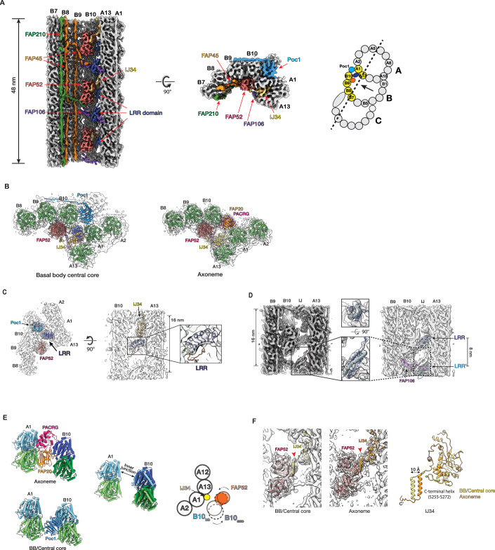
The cilium is a microtubule-based eukaryotic organelle critical for many cellular functions. Its assembly initiates at a basal body and continues as an axoneme that projects out of the cell to form a functional cilium. This assembly process is tightly regulated. However, our knowledge of the molecular architecture and the mechanism of assembly is limited. By applying cryo-electron tomography, we obtained structures of the inner junction in three regions of the cilium from Tetrahymena: the proximal, the central core of the basal body, and the axoneme. We identified several protein components in the basal body. While a few proteins are distributed throughout the entire length of the organelle, many are restricted to specific regions, forming intricate local interaction networks in the inner junction and bolstering local structural stability. By examining the inner junction in a POC1 knockout mutant, we found the triplet microtubule was destabilized, resulting in a defective structure. Surprisingly, several axoneme-specific components were found to "infiltrate" into the mutant basal body. Our findings provide molecular insight into cilium assembly at the inner junctions, underscoring its precise spatial regulation.

Keywords: Assembly; Basal Body; Centriole; Cilium; Electron Cryo-tomography.

Figure 1. Electron cryo-tomography structures of cilium inner junctions.

(A) A schematic diagram of a cilium in Tetrahymena, including BB and axoneme. The three regions in the BB, the proximal, central core, and distal, are highlighted in different green colors. Their approximate longitudinal spans are indicated. The three gray-colored cross-sections indicate the location of the structures presented in this work. (B) Left, schematic diagrams of the cross-section of the proximal, the central core region of the BB, and the axoneme. Right, representation of the triplet MT or doublet MT from the three regions. Distinct structures attached to the microtubule wall in each region, such as the cartwheel and the A–C linker in the proximal region, the inner scaffold in the central core region, and the Dynein complexes (ODA outer Dynein arm, IDA inner Dynein arm, DRC Dynein regulatory complex) and the radial spokes (RS) in the axoneme, are indicated. The red dashed line boxes highlight the A–B inner junctions (IJ). (C) Three representative subtomograms-averaged structures in 16-nm periodicity are presented in this work. From bottom to top are the proximal, the central core region of the BB, and the axoneme, as indicated in the cartoons in (B).

Figure 2. Structure of the inner junctions in the proximal region of the BB.

(A) Two orthogonal views of the A–B inner junction structure with 16-nm repeat. A FAP52-like MIP, FAP106, and Poc1 are colored in red, purple, and blue, respectively. A schematic diagram of TMT is on the right. The pfs shown in the structure are highlighted in yellow. A dash line indicates the cutting plane and an arrow indicates the direction of view. (B) Comparison of the A–B inner junctions in the BB’s proximal and central core regions. The proximal region structures are on the left, and the central core region structures are on the right. The MIP models and the tubulins (α-tubulins in green, β tubulin in light blue) are fit into the density maps in gray. Note a FAP52-like MIP binds to the B-tubule at a different location in the proximal region compared to the FAP52 in the central core region. (C) Upper: a composite map showing the A–B and B–C inner junctions in the proximal region. The A–B and B–C inner ladders crosslinking pfs A13-B10 and B7-C10 are highlighted in light pink and indicated by red arrowhead. A schematic diagram of TMT is on the right. The pfs shown in the structure are highlighted in yellow. The arrows indicate the directions of view in the bottom panels. Bottom: longitudinal cross-section views of the A–B and B–C inner junctions.

Figure 3. Structural changes at the transition from the proximal to the central core region of the BB.

(A) Focused classification on the subtomograms from the proximal region identifies two structures where a FAP52-like protein binds at different locations (indicated by red arrows). (B) The longitudinal distribution of the subtomograms from the proximal region. The 150 nm long proximal region is divided into 14 bins. Based on the two classes identified in (A), for each class, the number of subtomograms (y axis) found in each bin is plotted, showing their longitudinal distribution along the length of the proximal region (x axis). Right: A schematic diagram indicates the weighted average longitudinal location for Class 2 is at 130 nm. The weighted average length is $\mathrm{L}=\sum \mathrm{j}*\mathrm{Nj}/\sum \mathrm{Nj}$ (Nj: number of subtomograms found in bin j). (C) Left: The Class 2 average in a cross-section view. A red arrowhead indicates the A–B inner junction. A red dashed line and a black arrow indicate the cross-section and viewing direction of the structure on the right. Right: The averaged structure from Class 2, longitudinally spanning 70 nm. A yellow arrowhead indicates the location where the FAP52-like MIP (red arrowheads) shifting binding site. The shift coincides with the termination of the unidentified ladder-like protein in the A–B inner junction (red arrow). (D) Similar to (B), the longitudinal distribution of the subtomograms from the central core region. The 300 nm long central core region is divided into 28 bins. Based on the classification result shown in Fig. EV3C, the longitudinal distribution of subtomograms in Class 6 and the other five classes are plotted. The weighted average longitudinal position of Class 6 is at 170 nm from the very proximal end of the BB. This is illustrated in a schematic diagram on the right. (E) The averaged structure in Class 6 (Fig. EV3C) shows the changes of TMT transitioning from the proximal to the central core region. A red arrowhead indicates the inner scaffold. A red arrow indicates FAP52. A yellow arrowhead indicates the termination of the A–C linker and the emergence of the inner scaffold. (F) Mapping the distribution of subsets of subtomograms in the BB. Eight representative BBs are shown. Each dotted line represents a TMT, longitudinally spanning 450 nm from the proximal to the core region (an arrow indicates the polarity). The 450 nm longitudinal span is divided into 3 segments, each 150 nm long. The green dots represent the Class 1 subset in (A), an inner junction structure in the proximal region. The red dots represent subtomograms in Class 2 in (A) and EV3A, where a FAP52-like protein shift from pf B9 to FAP52 at the canonical position between pf B9 and B10. The blue dots represent Class 6 in (E) and EV3C, where the A–C linker recedes, and the inner scaffold emerges, marking the transition from the proximal to the central core region. The yellow dots represent the structure in the core region, where the A–C linker is absent, and the inner scaffold is fully assembled in the TMT.

Figure 4. Structure of the inner junctions in the central core region of the BB.

(A) Two orthogonal views of a 48-nm repeat structure at the A–B inner junction in the BB central core region. The MIPs are highlighted in different colors as indicated. On the right is a schematic diagram of the TMT where the pfs shown in the structure are highlighted in yellow. A dash line indicates the cutting plane and an arrow indicates the viewing direction of the structure on the left. (B) Comparing the A–B inner junction in a 16-nm repeat from the BB central core region to the axoneme. The MIP models and the tubulins (represented by α-tubulins in green) are fit into the density maps in gray. (C) A MIP with a leucine-rich repeat (LRR) motif in the A–B inner junction. An LRR model predicted by AlphaFold2 from the protein (UniProt: Q22N53) fits into the density map. The LRR motif makes potential interactions with pfs B10, A13, and A1 of the TMT wall, Poc1, and IJ34. (D) An AlphaFold 3 predicted model of a right-handed 4-helix bundle fits into the density map. It is formed by two NTDs from the neighboring LRR-containing proteins as an anti-parallel dimer. Each monomer is colored in either dark or light blue. (E) Comparing the inner junctions between the central core region and the axoneme. Left: the models of the inner junction in the central core of BB and the axoneme. Center: superposition of the two models using pf A1 as a reference. Pf B10 (α/β tubulin) in the BB central core are in light green and blue. Pf B10 (α/β tubulin) in the axoneme are in dark green and blue. Right: schematic illustration of the change. The solid circles represent the pf B10 and FAP52 from the BB central core region. The dashed circles represent the pf B10 and FAP52 in the axoneme. The two curved arrows indicate the movement of pf B10 and FAP52 from the central core to the axoneme. (F) Comparing the structures of IJ34 in the central core region and the axoneme. The left and center show that IJ34 and FAP52 fit into the density maps. Right: superposition of the two IJ34 using their main domains as a reference. Their C-terminal helices are 10 Å apart.

Figure 5. poc1Δ mutants destabilize the A–B inner junction and allow axonemal components to incorporate into the assembly.

(A) Upper: representative tomogram slices from poc1Δ BB show the TMTs split at the A–B inner junction at various longitudinal locations. Bottom: the blue lines highlight the split TMTs in the upper panels. The yellow arrows indicate the locations of the split. The minus ends of TMT are at the bottom, and the plus ends are at the top. Scale bar: 100 nm. (B) 3D classification of subtomograms from poc1Δ BB, focusing on the A–B inner junction. The resulting three subsets show structure variations at the A–B inner junction. In Class 1, the B-tubule is incomplete and detached from the A-tubule at the inner junction. In Class 2, the B-tubule is complete and remains attached to the A-tubule, though the Poc1 position is empty. In Class 3, the B-tubule is complete and connected to the A-tubule, while other proteins occupy the Poc1 site. Yellow dashed circles and arrows outline the position of Poc1 in the wild-type. The numbers indicate the number of particles in each class and their percentage in the dataset. An image from the wild-type and a schematic diagram is shown for comparison. (C) Further refinement of Class 3 at 8.0 Å identifies the FAP20/PACRG filament at the mutant BB’s inner junction gap. (D) Comparing the A–B inner junction in the central core region between wild-type and poc1Δ Class 3 shows an increased gap in the junction. Pf A1 is used as a reference for superposition. For Pf B10 (α/β tubulin), the wild-type is in light green and blue, and the poc1Δ is in dark green and blue. (E) Focused classification of subtomograms from poc1Δ BB (Class 3) identifies additional axonemal MIPs, CCDC81b, and BMIP1. Left, the mutant structure is shown in light green where the atomic models for CCDC81b/BMIP1 (PDB: 8V3I) are fit into the map. Right, the inner junction from the wild-type axoneme DMT is shown as a comparison. The corresponding MIPs CCDC81b/BMIP1, indicated by an arrow, are colored in lavender. (F) In poc1Δ BB, the LRR-motif MIP partially remains in the Class 2 average but is absent in Class 3, where the inner junction is occupied by FAP20/PACRG. For comparison, the wild-type BB structure is shown in gray. (G) Mapping the location of subtomogram from 3 subsets identified in the central core region of poc1Δ BBs. 8 representative BBs are shown. The green dots represent the Class 1 subset, an incomplete B-tubule detached from the A-tubule at the inner junction. The blue dots represent the Class 2 subset, complete B-tubule without Poc1. The red dots represent the Class 3 subset, the axoneme-like inner junction where FAP20/PACRG fills in the space left by Poc1. The arrows point in the direction from the proximal to the distal end of the BBs.

Figure 6. Summary of inner junction MIPs localized in different regions of BB and axoneme and their misplacement in the poc1Δ mutant.

(A) Schematic illustration summarizing the inner junction components in three regions of the cilium identified in this study. (B) A model illustrates the poc1Δ BB A–B inner junction partially morphing into an axoneme-like architecture. The double-ended arrows indicate the expansion of the inner junction gap once PACRG and FAP20 are incorporated. This causes disassociation of the LRR-motif MIP and facilitates the binding of axonemal components, such as CCDC81b and BMIP1. In the box, the axoneme-specific MIPs found in poc1Δ are indicated in red; note that many BB components are partially bound in the mutant as the inner junction structure is disrupted without Poc1.

Figure EV1. Related to Figs. 1, 2, 4, 5, S5. Assessing resolution of subtomogram averages by Fourier shell correlation (FSC).

The structures and their Fourier shell correlations as a function of resolution (1/Å) are reported in Table 2. (A) A 16-nm repeat of the A–B inner junction from the proximal region of BB (wild-type). (B) A 16-nm repeat of the B–C inner junction from the proximal region of BB (wild-type). (C) A 48-nm repeat of the A–B inner junction from the central core region of BB (wild-type). (D) A 16-nm repeat of the A–B inner junction from the central core region of BB (wild-type). (E) A 16-nm repeat of the A–B inner junction from the axoneme (wild-type). (F) A 16-nm repeat of the A–B inner junction from a subset (Class 3) of the central core region of poc1Δ BB. (G) A 48-nm repeat of the A–B inner junction from a subset (Class 3) of the central core region of poc1Δ BB.

Figure EV2. Related to Fig. 2. The inner junctions in the proximal region.

(A) Fitting the atomic models of FAP52, FAP106 and Poc1 into the 16-nm repeat averaged density map from the proximal region of BB. The FAP52 and FAP106 models are based on the axoneme structure (PDB: 8G2Z). The Poc1 model is from the AlphaFold2 database. (B) The maps of the A–B and B–C inner junctions in the proximal region of BB. The two unidentified proteins, namely the A–B inner ladder and B–C inner ladder crosslinking pfs A13-B10 or B7-C10, respectively, are highlighted in light pink and indicated by red arrowheads. On the right, a schematic diagram shows the location of the above two maps in the TMT. Black arrows indicate the viewing directions. (C) 3D Classification of the subtomograms from the proximal region of poc1Δ TMT identified a small fraction of the dataset (8%) having complete TMT, where the two unidentified proteins, the A–B inner ladder and B–C inner ladder indicated by red arrowheads, remain in the inner junctions. The number of subtomograms in each class is shown. The dashed circles in the cartoon indicate the location of Poc1 in the wild-type.

Figure EV3. Related to Fig. 3.

(A) Focused 3D classification on the subtomograms from the proximal region of the BB. A yellow dashed circle indicates the focused area centered on the inner junction. Yellow or red arrowheads indicate the locations of FAP52 in the class averages. (B) A Longitudinal cross-section of the A–B inner junction showing the FAP52, indicated by red arrowheads, shifts binding from pf B9 to pf 9/10. A schematic illustration of the TMT is on the right. A dashed line and an arrow indicate the cross-section and the viewing direction of the structure on the left. A red dot represents FAP52. (C) Focused 3D classification on the subtomograms from the central core region of the BB. The Class 6 is highlighted with a red frame. In this class, the A–C linker and the inner scaffold are indicated by yellow arrowheads. The number of subtomograms in each group is provided.

Figure EV4. Related to Fig. 4.

(A) Fitting the atomic models of MIPs found in the central core region of BB into the averaged density map. Each inset shows the fitting of a MIP model into its local density and its surroundings. In the “FAP210” inset panel, a red asterisk indicates a potential interaction between FAP210 and FAP52 that has been observed previously in the axoneme structure. In the “FAP52” inset panel, a black arrow indicates a potential interaction between FAP52 and FAP106. The α/β tubulins are colored in pale green and blue in the background. The 16-nm repeat map from the central core region is used for fitting of FAP52. FAP106, IJ34, and Poc1 models, as these MIPs have 16-nm or 8-nm (Poc1) periodicity. (B) A cross-section slice of the density map shows an LRR motif highlighted in a red dashed line square. (C) An AlphaFold2 predicted protein structure (UniProt Q22N53) was identified previously in the BB proteome. The protein is composed of a N-terminal α-helix hairpin (NTD) and a C-terminal LRR motif (CTD). The structure is colored based on the prediction confidence score (pLDDT: the predicted local distance difference test). The high confidence is in dark blue, while the low confidence is in yellow or orange. (D) An AlphaFold 3 predicted 4-helix bundle formed by dimerizing two NTD/hairpins. Two copies of the NTD hairpin from the LRR-motif MIP (UniProt Q22N53) form an anti-parallel dimer. One monomer is in dark blue (Helix 1 and Helix 2) and the other monomer is in light blue (Helix 1’ and Helix 2’). The dimer forms a right-handed 4-helix bundle. (E) The predicted aligned error (PAE) plot provides inter-domain packing confidence scores. The dark and light blue imply the prediction with high confidence, while the gray and white indicate low confidence in the interaction. On the right, a ChimeraX-adapted color scheme is used where the 4-helix bundle is colored based on the PAE potential interaction score. The two N-terminal helices (Helix 1, Helix 1’) are in cyan, and the two C-terminal helices (Helix 2 and Helix 2’) are in magenta, indicating that the interaction between Helix 1 and Helix 1’ (cyan), Helix 2 and Helix 2’ (magenta) are with high confidence. (F) Inter-protofilament angle measurement. Left: the angles between pfs B9 and B10 are measured at the three regions, showing the variation of local curvature. The FAP52 and Poc1 or FAP20/PACRG are shown as reference points. Right: a schematic diagram depicts the inter-protofilament angles at the A–B inner junction. More complete measurements are in Table 1.

Figure EV5. Related to Fig. 5. Comparing the inner junctions between the wild-type axoneme and the Class 3 from the poc1Δ BBs.

(A) Comparing the two structures in two orthogonal views, the wild-type axoneme is in gray, and the poc1Δ BB is in green. (B) Fitting the molecular models into the density maps in (A). The α/β tubulins are in light green and blue, FAP20 is in orange, and PACRG is in dark magenta. The arrows indicate the A–B inner junctions. (C) Comparing the 48-nm repeat from the wild-type axoneme (left) and from a subset of poc1Δ BB (Class 3, on the right in green). The 48-nm repeat average from a subset of poc1Δ BB (Class 3) shows nearly identical structure to the wild-type axoneme inner junction. This is the same subset/class as shown in Fig. 5E, but the longitudinal length is extended to 48 nm here. For clarity, the poc1Δ BB mutant map is low-pass filtered to 12 Å.

References

1. Abramson J, Adler J, Dunger J, Evans R, Green T, Pritzel A, Ronneberger O, Willmore L, Ballard AJ, Bambrick J et al (2024) Accurate structure prediction of biomolecular interactions with AlphaFold 3. Nature 630:493–500 - PMC - PubMed
1. Allen RD (1969) The morphogenesis of basal bodies and accessory structures of the cortex of the ciliated protozoan Tetrahymena pyriformis. J Cell Biol 40:716–733 - PMC - PubMed
1. Arslanhan MD, Cengiz-Emek S, Odabasi E, Steib E, Hamel V, Guichard P, Firat-Karalar EN (2023) CCDC15 localizes to the centriole inner scaffold and controls centriole length and integrity. J Cell Biol 222:e202305009 - PMC - PubMed
1. Bharat TAM, Scheres SHW (2016) Resolving macromolecular structures from electron cryo-tomography data using subtomogram averaging in RELION. Nat Protoc 11:2054–2065 - PMC - PubMed
1. Breugel M, van, Hirono M, Andreeva A, Yanagisawa H, Yamaguchi S, Nakazawa Y, Morgner N, Petrovich M, Ebong I-O, Robinson CV et al (2011) Structures of SAS-6 Suggest Its Organization in Centrioles. Science 331:1196–1199 - PubMed