The Boynton Illusion: Chromatic edge attraction to a luminance contour

Abstract

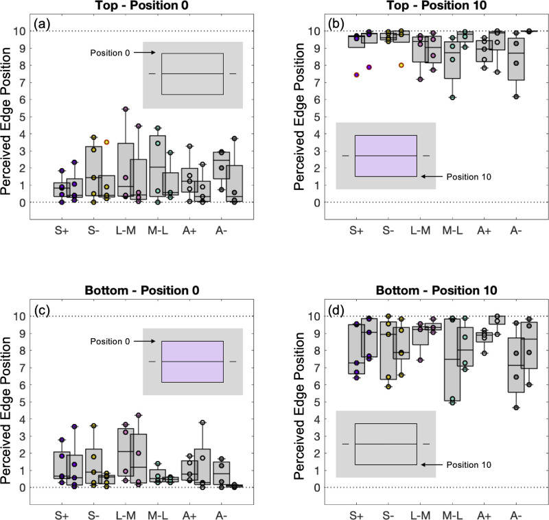
In the Boynton Illusion, the perceived location of a low-contrast chromatic edge is altered by a nearby high-contrast luminance contour. Our study explores this color spreading effect across different chromatic directions using a position judgment task. We used the gap effect stimulus, which consists of a box evenly divided by a central contour, in half of the conditions. The suprathreshold chromatic test area embedded in the box provided a horizontal chromatic edge parallel to the central, high-contrast luminance contour that varied in its distance from the contour. An attraction effect of the nearest high-contrast contour on low-contrast chromatic and achromatic edges was observed. Specifically, when the test area is smaller than the region defined by the outer and middle contours, the edge is perceived to be closer to the middle contour (the colored area is perceived to be larger), a filling-in effect; conversely, when the test area extends beyond the middle contour, the edge is perceived to be closer to the middle contour (the colored area is perceived to be smaller), indicating a filling-out of color. Achromatic directions exhibit a relatively smaller effect than chromatic directions, whereas S-cone and equiluminant red and green edges show the same magnitude of positional displacement. The results can be interpreted as the visual system attempting to assign a single hue or brightness to a demarcated region.

Figure 1.

Gap effect. (a) Two colored regions are juxtaposed. (b) A gap is added between two colored regions which enhances the discriminability between the fields (Boynton et al., 1977).

Figure 2.

Illustration of the Boynton Illusion. The yellow areas on the left and right are same squares. With a black squiggly contour drawn on top of the right square, the yellow edge appears to be defined by the black contour when viewing from a certain viewing distance.

Figure 3.

Stimuli in all experimental conditions with the S+ chromaticity. The top panel shows no-contour stimulus (left) and with-contour stimulus (right) in the contrast detection task. The chromatic area in both conditions fills in the top half of the rectangular box. The bottom panel shows examples of the no-contour and with-contour stimuli in Top and Bottom conditions in Experiment 2, the position judgment task.

Figure 4.

Box-and-whisker plot of threshold ratio of no-contour stimulus and with-contour stimulus for six chromatic conditions. The magenta symbols represent the log detection ratios for each observer, with different symbols used to distinguish between observers' data. Each boxplot displays a median marked by a central line and quartiles at the 25th and 75th percentiles. Whiskers extend to the maximum non-outlier points. Outliers falling more than 1.5 times the interquartile range from the closest quartile are indicated with black crosses.

Figure 5.

Stimuli in the position judgment experiment. For each test rectangle, nine vertical positions were defined from Top to Bottom to indicate the location of the test edge. The Top and Bottom conditions are shown at left and right, respectively. The chromatic edge position is at “4” in the Top condition, and “6” in the Bottom condition. Two additional conditions, with no chromatic stimulus, were coded as being at position 0 or position 10. For data analysis, position responses in the Bottom condition were subtracted from 10 (see text). The dashed gray arrows and the columns of numerals were not present in the actual experiment, but solid black line segments did mark the middle of the box in every presentation (shown clearly on the right of each panel, but obscured by the gray arrow on the left).

Figure 6.

Illustrative results of one observer in one color condition (S+). Curves in the left panels show the perceived edge position against the real edge position and curves in the right panels show the effect of adding a middle contour (with-contour minus no-contour positions), in terms of visual angle and percentage of box height. The gray quadrants represent responses showing that the edge was perceived closer to the middle position when there was a contour there. Panels are shown, from Top to Bottom, in the order of the Top condition, the Bottom condition, and the average of the two conditions. Error bars in the left panels represent standard errors, and error bars in the right panels represent standard deviations calculated with the propagation of error method. Note that data points at position 0 and position 10 are forced to converge to the diagonals for better visualization of the filling-in effect; the actual responses at those blank positions are described later in this section.

Figure 7.

Illustration of the filling-in pattern of the chromatic edge in different conditions. Left and right panels show the Top and Bottom conditions, and left and right columns in each panel are no-contour and with-contour conditions, respectively. The chromatic edge is perceptually-attracted to the nearest contour in all cases.

Figure 8.

The effect of adding the contour in six color conditions, averaged across observers and Top and Bottom conditions. Error bars are standard deviations averaged across observers derived using the propagation of error method. An illustration of the attraction effect of the middle contour is shown in the second and fourth quadrants of the top left panel. Panels S+, S–, and A+ show the average of all five observers, whereas the other panels show the average of four observers (one observer did not complete all conditions). See text for description of the dashed curves.

Figure 9.

Box-and-whisker plot for corrected d’ (left) and λ_center (right), with the correction being applied to deal with cases with no false alarms or 100% hits (Hautus, 1995; see the Appendix). For each color direction in each panel, the boxplots for the with-contour condition are on the left and the no-contour condition data are slightly shifted to the right. Colored circles correspond to the d’ or λ_center of each observer, with the median for each color direction represented as the central line. The top and bottom bounds of the gray boxes indicate the 75th and 25th percentiles, respectively. Outliers, points that lie beyond 1.5 × the interquartile range, are outside of the whiskers; the whiskers themselves indicate the maximum and minimum values within that 1.5 × interquartile range.

Figure A1.

Judgment bias at positions 0 and 10. The four panels show the four conditions where either no chromatic rectangle was presented, or the chromatic rectangle filled the box and its edge was overwritten by the box contour. The corresponding with-contour stimulus and judgment position are shown in each panel. The box-and-whisker plots show the median, the upper and lower quantiles, the non-outlier minimum and maximum values, and the outliers (data points with red outlines that are more than 1.5 × the interquartile range above and below the box). For each color direction in each panel, the boxplots for the with-contour condition are on the left and the no-contour condition data are slightly shifted to the right.

References

1. Badcock, D. R., & Westheimer, G. (1985). Spatial location and hyperacuity: the centre/surround localization contribution function has two substrates. Vision Research , 25(9), 1259–1267, doi:10.1016/0042-6989(85)90041-0. - DOI - PubMed
1. Blakeslee, B., Cope, D., & McCourt, M. E. (2016). The Oriented Difference of Gaussians (ODOG) model of brightness perception: Overview and executable Mathematica notebooks. Behavior Research Methods , 48(1), 306–312, doi:10.3758/s13428-015-0573-4. - DOI - PMC - PubMed
1. Blakeslee, B., & McCourt, M. E. (2008). Nearly instantaneous brightness induction. Journal of Vision , 8(2),15, 11–18, doi:10.1167/8.2.15. - DOI - PMC - PubMed
1. Boynton, R. M. (1980). Design for an eye . In McFadden D. (Ed.), Neural mechanisms in behavior (pp. 38–72). Springer-Verlag.
1. Boynton, R. M., Hayhoe, M. M., & MacLeod, D. I. A. (1977). The gap effect: chromatic and achromatic visual discrimination as affected by field separation. Optica Acta: International Journal of Optics , 24(2), 159–177, doi:10.1080/713819496. - DOI
Publication types
LinkOut - more resources