From Foreshock 30-Second Waves to Magnetospheric Pc3 Waves

Abstract

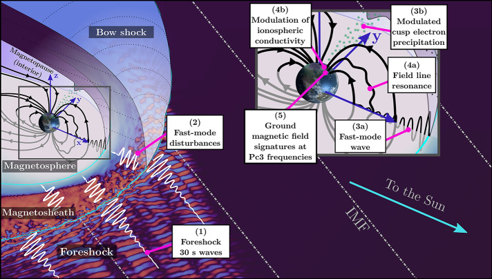
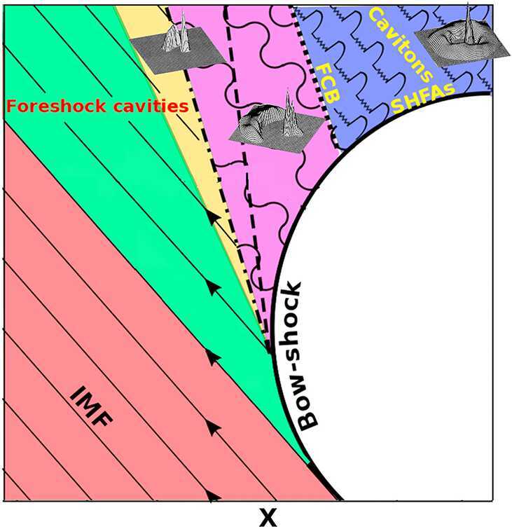
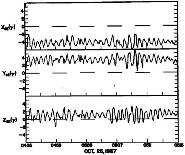
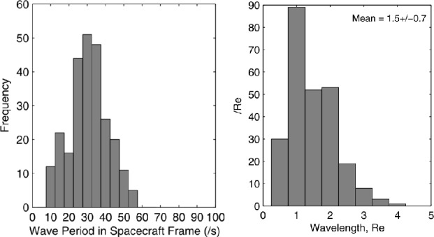
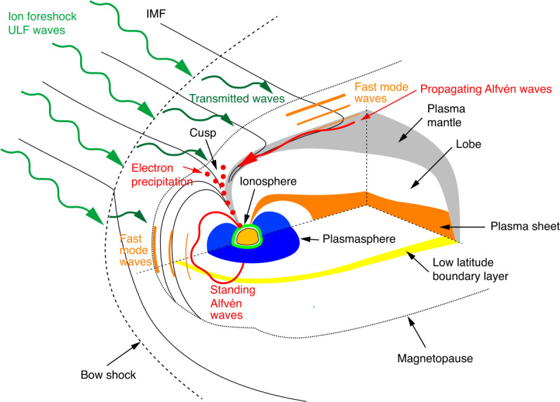
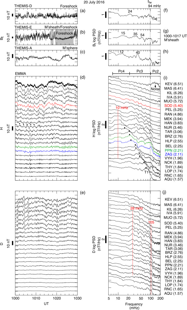
Ultra-low frequency waves, with periods between 1-1000 s, are ubiquitous in the near-Earth plasma environment and play an important role in magnetospheric dynamics and in the transfer of electromagnetic energy from the solar wind to the magnetosphere. A class of those waves, often referred to as Pc3 waves when they are recorded from the ground, with periods between 10 and 45 s, are routinely observed in the dayside magnetosphere. They originate from the ion foreshock, a region of geospace extending upstream of the quasi-parallel portion of Earth's bow shock. There, the interaction between shock-reflected ions and the incoming solar wind gives rise to a variety of waves, and predominantly fast-magnetosonic waves with a period typically around 30 s. The connection between these waves upstream of the shock and their counterparts observed inside the magnetosphere and on the ground was inferred already early on in space observations due to similar properties, thereby implying the transmission of the waves across near-Earth space, through the shock and the magnetopause. This review provides an overview of foreshock 30-second/Pc3 waves research from the early observations in the 1960s to the present day, covering the entire propagation pathway of these waves, from the foreshock to the ground. We describe the processes at play in the different regions of geospace, and review observational, theoretical and numerical works pertaining to the study of these waves. We conclude this review with unresolved questions and upcoming opportunities in both observations and simulations to further our understanding of these waves.

Fig. 1

Overview of near-Earth space, with the main steps of the transmission pathways of foreshock 30-second waves: (1) generation in the foreshock, (2) transmission through the magnetosheath, (3) entry into the magnetosphere in the equatorial region as fast-mode waves (3a) coupling with field line resonances (4a) and at high latitudes via modulated precipitation (3b) resulting in variations of the ionospheric conductivity (4b), eventually leading to (5) the observations of Pc3 pulsations on the ground

Fig. 2

Regions in the near-Earth environment and associated ion populations. The green, yellow, purple and blue colors represent regions magnetically connected to the bow shock. The ion and ULF wave foreshocks are colored in purple and blue. Superposed are three panels exhibiting examples of field-aligned (Fairfield ; Paschmann et al. 1980), intermediate (Argo et al. ; Meziane and d’Uston 1998) and diffuse (Paschmann et al. ; Bonifazi and Moreno ,; Winske and Leroy 1984) ion distributions that coexist with narrow-peaked solar wind ion distributions. Adapted from Kajdič et al. (2017) and Paschmann et al. (1981)

Fig. 3

Large-amplitude quasi-sinusoidal waves with a period around 30 s on the three magnetic field components measured by the Explorer 34 spacecraft in the Earth’s foreshock. The waves were observed about $14R_{\mathrm{E}}$ from the average bow shock position. Figure reproduced with permission from Fairfield (1969), copyright by the AGU

Fig. 4

Histograms of the wave periods in the spacecraft frame and of the wavelengths of 30-second waves observed by the Cluster spacecraft during 255 2-min intervals in the foreshock in 2001. The wave period was determined from the average autocorrelation of the time series and the wavelength based on timing analysis between the four-spacecraft measurements. Figure adapted and reproduced with permission from Eastwood et al. (2005a), copyright by the AGU

Fig. 5

Refraction of the foreshock wave fronts as they are advected through regions of different suprathermal ion density and velocity, in a global 2D hybrid-Vlasov simulation with a quasi-radial IMF geometry. The white arrow tracks a single wave front at different times in the simulation. Figure reproduced with permission from Palmroth et al. (2015), copyright by the AGU

Fig. 6

Examples of sinusoidal transverse ULF waves (top) and shocklets (bottom) in the Earth’s foreshock. Figure adapted from Greenstadt et al. (1995), reproduced with permission from COSPAR, copyright by Elsevier

Fig. 7

Observations of a single short large-amplitude magnetic structure (SLAMS) by two space missions. Figure reproduced with permission from de Wit et al. (1999), copyright by the AGU

Fig. 8

Bending of magnetic field lines at the shock transition in local hybrid simulations by Krauss-Varban et al. (2008). Figure reproduced with permission from Krauss-Varban et al. (2008), copyright by AIP Publishing

Fig. 9

Power spectra of the waves upstream and downstream of the shock in a 1-D local hybrid-PiC simulations performed by Krauss-Varban (1995). From Krauss-Varban (1995), reproduced with permission from COSPAR, copyright by Elsevier

Fig. 10

Simulation results for 4 out of 11 local hybrid runs from Kajdič et al. (2021) at times when the shock was located in the middle of the simulation domain. Colours represent the magnetic field magnitude. ${\theta }_{\mathrm{Bn}}$ increases from left to right while the shock’s Alfvénic Mach number (${\mathrm{M}}_{\mathrm{A}}$) increases from top to bottom. The shocks on panels a, c and d are classified by Kajdič et al. (2021) as weakly rippled, while the shock on panel b is strongy rippled. Figure adapted and reproduced with permission from Kajdič et al. (2021), copyright by the AGU

Fig. 11

Total pressure variations in the magnetosheath caused by the foreshock waves. Time-position maps of the magnetosonic Mach number (a) and the total pressure (b) along the Sun-Earth line. The total pressure is calculated as the sum of the thermal pressure and the magnetic pressure. The white contour marks where ${\mathrm{M}}_{\mathrm{ms}}=1$. From Turc et al. (2023)

Fig. 12

Average magnetic field parallel and transverse standard deviations as a function of magnetic local time (denoted here as $\mathrm{\Phi }$), measured in the magnetosheath by the ISEE 2 spacecraft between October 1977 and October 1979. The data are separated into four cone angle bins, showing an enhanced level of fluctuations for low cone angle values. Figure reproduced with permission from Luhmann et al. (1986), copyright by the AGU

Fig. 13

Flowlines of the magnetosheath plasma as a function of the IMF cone angle, for radial IMF (${\theta }_{\mathrm{Bx}}=0$, left) and Parker spiral IMF orientation (${\theta }_{\mathrm{Bx}}={45}^{\circ }$, right), in the plane containing the IMF and solar wind velocity and passing through the subsolar point. The labels of the flowlines correspond to the ${\theta }_{\mathrm{Bn}}$ value encountered upon crossing the bow shock. Figure adapted and reproduced with permission from Russell et al. (1983), copyright by the AGU

Fig. 14

Direction of propagation of the dominant wave modes upstream and downstream of the bow shock, based on a statistical survey of Cluster data. From Narita and Glassmeier (2006)

Fig. 15

Dynamic power spectra of the total magnetic field fluctuations observed by the THEMIS-D (foreshock) and THEMIS-E (magnetosheath and foreshock) spacecraft during a period of quasi-radial IMF. The black curve indicates the expected foreshock wave frequency based on the Takahashi et al. (1984) formula. Figure adapted and reproduced with permission from Takahashi et al. (2021), copyright by the AGU

Fig. 16

MMS observations during a one-hour interval when the spacecraft crossed from the foreshock into the subsolar magnetosheath. The top panels show (a) the magnetic field magnitude and electron density and (b) the magnetic field GSE components. The bottom part of the figure shows close-up of two intervals in the foreshock (left) and the magnetosheath (right), marked by the solid and dashed lines in the top panels. Shown in the bottom panels are the cross-correlation between the density and magnetic field strength fluctuations (c and f), the wavelet trace power spectra (d and g) and the compressibility of the magnetic fluctuations (e and h). The white dotted-dashed curves indicate the expected foreshock wave frequency based on the Takahashi et al. (1984) formula. From Turc et al. (2023)

Fig. 17

Illustration of wave entry from different locations on the magnetosheath-magnetosphere boundary. This is a composite of Fig. 1.18 of Kivelson and Russell (1995) and Fig. 7 of Chugunova et al. (2004)

Fig. 18

(a) Magnetic pulsations recorded at the Petropavlovsk Kamchatsky magnetometer station on two different days. The arrows indicate the direction of the IMF in the ecliptic plane, with the Sun in the upward direction. (b) Occurrence of Pc3 pulsations as a function of the IMF cone angle. Figure reproduced with permission from Troitskaya (1994), copyright by the AGU

Fig. 19

Amplitude of the Pc3 fluctuations recorded by ground-based magnetometers as a function of the $L$ value of the station, for 5 different events. The Pc3 wave amplitudes are obtained by integrating under the peak of the wave power spectra. The wave amplitude tends to increase when moving to larger $L$ values. Figure reproduced with permission from Odera et al. (1994), copyright by the AGU

Fig. 20

Schematic of the field line resonance process driven by fast-mode waves propagating from the magnetopause inwards

Fig. 21

Diurnal variation of Pc3 (thick line) and Pc4 (thin line) hourly pulsation energy W [${\mathrm{nT}}^2/\mathrm{mHz}$] of the magnetic field H component measured at four high-latitude ground stations in Antarctica. The latitudes of the stations in corrected geomagnetic coordinates are indicated on top of each of the panels and correspond to auroral latitudes (P3), cusp latitudes (P4 and P6) and polar cap (P5). Reproduced with permission from Pilipenko et al. (2008), copyright by Elsevier

Fig. 22

Simultaneous observations of Pc3 waves at polar and low latitudes, at the expected foreshock wave frequency (blue line). The panels show the dynamic signal-to-noise ratio R of the fluctuations of the magnetic field horizontal components (H and D) recorded on 15 February 2009 at different magnetometer stations: Dome C (DMC) and Terra Nova Bay (TNB), in Antarctica, on open field lines, and Nagycenk (NCK; Hungary) and Castello Tesino (CST; Italy), on low-latitude, closed field lines. From Regi et al. (2014)

Fig. 23

Long-term statistics of the frequencies of ground magnetic pulsations detected $L=1.6$. (a) Dominant frequencies ($\widetilde{f_r}$ and $f_D$) and a model foreshock wave frequency ($\overline{f_{\mathrm{u}}}$) derived from the annual mean of the magnitude of IMF. (b) Sunspot number. Figure reproduced with permission from Vellante et al. (1996), copyright by the AGU

Fig. 24

Schematic of propagation of an MHD impulse from a point source located on the magnetopause. Figure reproduced with permission from Takahashi and Heilig (2019), copyright by the AGU

Fig. 25

$L$ versus structure of magnetic field perturbation observed by the European quasi Meridian magnetometer array (EMMA). Figure reproduced with permission from Takahashi and Heilig (2019), copyright by the AGU

Fig. 26

Distribution of the mean Pc3 compressional wave power measured in the topside ionosphere by the CHAMP spacecraft, as a function of MLT and magnetic latitude. The different populations of Pc3 waves, at equatorial and high latitudes, and on the dayside and the nightside, can clearly be seen from this figure. From Heilig et al. (2007)

Fig. 27

Example of multiharmonic toroidal waves observed by Van Allen Probe A. (a) IMF cone angle according to the solar wind OMNI data. (b) Dynamic spectra of the magnetic field compressional component at Van Allen Probe A. (c) Dynamic spectra of the magnetic field azimuthal component. (d) Frequencies of toroidal waves determined from the magnetic field spectra (blue) and electric field spectra (red). The labels T1, T2,.. indicate the harmonic mode number. The spacecraft location is given at the bottom. This figure combines panels selected from Figs. 3, 4, and 6 of Takahashi et al. (2015), reproduced with permission from Takahashi et al. (2015), copyright by the AGU

Fig. 28

Simultaneous observations of compressional Pc3 waves in the dayside outer magnetosphere and daytime auroral pulsations on the ground. (a) Location of three THEMIS probes and the projection of South Pole Station (SPA) onto the equatorial plane. (b) IMF components and cone angle upstream of the Earth’s bow shock from the OMNI data set. (c) Magnetic field strength measured by the THEMIS-A spacecraft and its associated dynamic power spectrum. (d) Auroral luminosity measured at SPA and its associated dynamic power spectrum. The white circles on the dynamic power spectra correspond to the expected frequency for the foreshock waves, estimated using the Takahashi et al. (1984) formula. Figure reproduced with permission from Motoba et al. (2019), copyright by the AGU

Fig. 29

Ion differential fluxes for the ${90}^{\circ }$ pitch angle helium ions (top) and power spectrum of the parallel magnetic field component (bottom) measured by Van Allen Probe A. A clear anti-correlation can be see between the He ion fluxes and the wave power. From Kim et al. (2017)

Fig. 30

IMF cone angle distribution during magnetic clouds arriving at Earth’s orbit during 2000–2014. Figure reproduced with permission from Turc et al. (2016), copyright by the AGU

Fig. 31

Comparison of foreshock 30-second wave properties during quiet solar wind conditions (left) and magnetic cloud events (right), showing a higher and more variable wave frequency when the IMF strength is enhanced. Figure reproduced with permission from Turc et al. (2019), copyright by the AGU

Fig. 32

Magnetic field measurements and associated power spectra of the fluctuations from the THEMIS-D (foreshock), THEMIS-E (magnetosheath and foreshock), and THEMIS-A (dayside magnetosphere) satellites, and from magnetometers from the EMMA network (ground). The ground-based measurements strongly differ from the upstream observations, showing in particular no clear peak at the foreshock wave frequency (94 mHz). Figure reproduced with permission from Takahashi et al. (2021), copyright by the AGU

Fig. 33

Pc3 wave power observed on the ground between 2001 and 2007, as a function of (a) solar wind velocity, (b) solar wind density, (c) Alfvén and (d) magnetosonic Mach number. Adapted from Heilig et al. (2010)

Fig. 34

Large-amplitude ULF waves with period of $\sim 20$ s in the foreshock and magnetosheath of Venus observed by the Venus Express satellite on 26 July 2011. Figure reproduced with permission from Shan et al. (2014), copyright by the AGU

Fig. 35

Examples of magnetic field measurements upstream and downstream of quasi-parallel interplanetary shocks observed by the STEREO spacecraft, showing prominent, mostly transverse ULF waves in the upstream of the shocks. Figure reproduced with permission from Blanco-Cano et al. (2016), copyright by the AGU

Fig. 36

Field-line resonances in the magnetosphere of Ganymede, observed during the G8 and the G28 Galileo flybys. The top panels show one of the transverse magnetic field components and the bottom panels the associated power spectra. The red and green bars in the bottom panels indicate the first and second harmonics and the horizontal lines depict the 95% confidence level. From Volwerk et al. (2013)

Fig. 37

Dayside conjunction of the Cluster, MMS and THEMIS missions on 27 February 2022. The approximate magnetopause (solid black line) and bow shock (dashed black line) positions are determined using the Shue et al. (1998) and Merka et al. (2005) models, respectively, using the average solar wind parameters between 12:00 and 23:59 UT on 27 Feb 2022

References

1. Ala-Lahti MM, Kilpua EKJ, Dimmock AP, Osmane A, Pulkkinen T, Souček J (2018) Statistical analysis of mirror mode waves in sheath regions driven by interplanetary coronal mass ejection. Ann Geophys 36(3):793–808
1. Ala-Lahti M, Kilpua EKJ, Souček J, Pulkkinen TI, Dimmock AP (2019) Alfvén ion cyclotron waves in sheath regions driven by interplanetary coronal mass ejections. J Geophys Res Space Phys 124(6):3893–3909
1. Ala-Lahti M, Dimmock AP, Pulkkinen TI, Good SW, Yordanova E, Turc L, Kilpua EKJ (2021) Transmission of an ICME sheath into the Earth’s magnetosheath and the occurrence of traveling foreshocks. J Geophys Res Space Phys 126(12):e29896
1. Anderson BJ, Engebretson MJ (1995) Relative intensity of toroidal and compressional Pc 3-4 wave power in the dayside outer magnetosphere. J Geophys Res 100(A6):9591–9604
1. Anderson BJ, Fuselier SA (1993) Magnetic pulsations from 0.1 to 4.0 Hz and associated plasma properties in the Earth’s subsolar magnetosheath and plasma depletion layer. J Geophys Res 98(A2):1461–1480
LinkOut - more resources