Observation of first- and second-order dissipative phase transitions in a two-photon driven Kerr resonator

Abstract

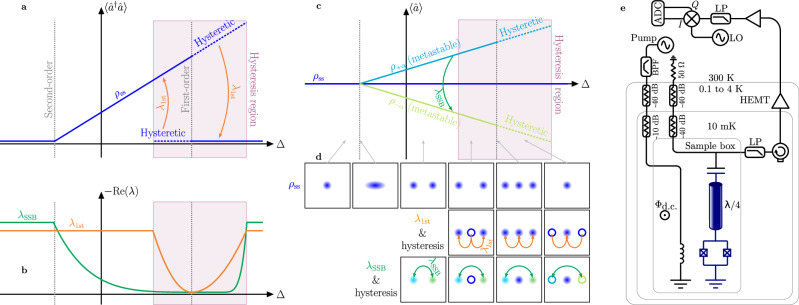
In open quantum systems, dissipative phase transitions (DPTs) emerge from the interplay between unitary evolution, drive, and dissipation. While second-order DPTs have been predominantly investigated theoretically, first-order DPTs have been observed in single-photon-driven Kerr resonators. We present here an experimental and theoretical analysis of both first and second-order DPTs in a two-photon-driven superconducting Kerr resonator. We characterize the steady state at the critical points, showing squeezing below vacuum and the coexistence of phases with different photon numbers. Through time resolved measurements, we study the dynamics across the critical points and observe hysteresis cycles at the first-order DPT and spontaneous symmetry breaking at the second-order DPT. Extracting the timescales of the critical phenomena reveals slowing down across five orders of magnitude when scaling towards the thermodynamic limit. Our results showcase the engineering of criticality in superconducting circuits, advancing the use of parametric resonators for critically-enhanced quantum information applications.

Fig. 1. Sketch of the theory of dissipative phase transitions and of the experimental set-up.

a Illustration of dissipative phase transitions (DPTs) according to Ref. Sweeping a the pump-resonator detuning Δ, the photons in the resonator $⟨{\widehat{a}}^{†}\widehat{a}⟩$ (blue curve) changes discontinuously (first-order DPT), or continuously with non-continuous derivative (second-order DPT). The blue dashed lines indicate the metastable states associated with hysteresis across the first-order DPT, and the purple rectangle marks the hysteresis region. b The Liouvillian gaps λ_SSB in green (λ_1st in orange) associated with the second-order (first-order) DPT. c Throughout the detuning sweep $⟨\widehat{a}⟩=0$ (blue curve). However, after second-order transition, the states ρ_±α shown in light blue and green, become metastable, with switching rate λ_SSB. The dashed lines indicate the metastable states associated with hysteresis across the first-order DPT. d Phase-space-like representation of the system across the DPTs. The top, middle, and bottom rows respectively represent the steady state (blue), the metastable state associated with λ_1st (hollow blue), and the metastable states associated with λ_SSB. The arrows within each panel indicate the decay of an initial state towards the steady state. The green arrows represent the decay of a non-symmetric state at a rate λ_SSB. The orange arrows are associated with the metastable state of the first-order DPT, decaying at a rate λ_1st. e Schematic illustrating the device and the experimental setup. The device is a hanger-type λ/4 coplanar waveguide resonator. The right side of the feedline is used to collect the emitted signal via heterodyne detection, whereas the left side is only used for spectroscopy measurements to extract the device parameters and is otherwise terminated by 50 Ω (see Supplementary Note 2). The other side of the cavity is terminated to ground via a SQUID. A magnetic field is applied through the SQUID, tuning both the resonance frequency and the Kerr nonlinearity. A second waveguide, inductively coupled to the SQUID, is used to supply a coherent pump tone around twice the resonant frequency of the cavity (ω_p ≃ 2ω_r). The pump results in a two-photon drive for the cavity^,.

Fig. 2. Characterization of the steady state.

a Phase diagram showing the number of photons in the resonator as a function of the detuning Δ and input power, obtained by heterodyne detection of the emitted field. The three phases are indicated by: (i) square marker (the vacuum at negative detuning); (ii) hexagon marker (the bright phase); (iii) pentagon marker (the vacuum at positive detuning). The passage between these phases is accompanied by a second- [(i)→(ii), circle marker] and first-order DPTs [(ii)→(iii), triangle marker]. b Rescaled number of photons ${\tilde{n}}_{\mathrm{s}s}=n_{\mathrm{s}s}/L$ as a function of the rescaled detuning $\tilde{\mathrm{\Delta }}=\mathrm{\Delta }/L$ and rescaled drive $G=\tilde{G}L$ for increasing scaling parameter L, with $\tilde{G}=65.5$ KHz (see also text and Methods for details). Circles indicate the experimental data, and solid lines are obtained from the numerical simulation of Eq. (2). The emergent discontinuities at negative and positive detuning with increasing L signal the presence of a second- and first-order DPT in the thermodynamic limit, respectively. c Higher-resolution characterization of the abrupt change in ${\tilde{n}}_{\mathrm{s}s}$ across the first-order DPT. The error bars correspond to the standard deviation over 4 experiments. d Husimi-Q function estimated through heterodyne detection. The markers correspond to those in (a), and the values of $\tilde{\mathrm{\Delta }}$ corresponds to the vertical dotted gray lines in (b). e Histogram of the measured phase Φ for L = 1.41. f Bimodality coefficient (i.e., Binder cumulant) B(Φ), defined in the main text, as a function of rescaled detuning $\tilde{\mathrm{\Delta }}$ for increasing scaling parameter L. Crossing of the cumulant corresponds to the critical points.

Fig. 3. Squeezing at the second-order DPT.

Rescaled photon number (a), its first (b), and second derivatives (c) calculated from the experimental data as a function of detuning. d The squeezing level $S=-10\log \left(\mathrm{\Delta }{x}_{\varphi }^2/0.5\right)$ evaluated across the second-order DPT. Notice that the maximum is in the vicinity of the critical point indicated by the maximum of the second derivative of the photon number in (c). The vertical dotted line indicates the expected maximum of the squeezing parameter obtained by numerical simulation of the steady state. The colored shaded region in (c) and the error bars in a represent the standard deviation calculated from 100 bootstrapped dataset of the measured data (see “Method for details).

Fig. 4. Analysis of the second-order DPT.

a A segment of the measured quadrature. As a function of time, we plot I(t) for L = 1.41 at various rescaled detunings $\tilde{\mathrm{\Delta }}=\mathrm{\Delta }/L$, indicated by the marker in each panel. Random jumps between two opposite values of the quadrature occur as time passes. These correspond to the switches between the states ${\rho }_{\mathrm{SSB}}^{+}$ and ${\rho }_{\mathrm{SSB}}^{-}$, as described in the main text. Using the entire collected signal, we recover a bimodal Husimi function shown on the right. b The autocorrelation function C_ss(t) (see Eq. (3) and “Methods”), obtained from a single measurement trace as those shown in panel a. The markers at the end of the curves represent the values of $\tilde{\mathrm{\Delta }}$, and the colors indicate the scaling parameter (L = 1.29: purple, L = 1.41: red). The Liouvillian gap can be extracted from fitting these curves using Eq. (3). The fits are represented by the black lines. c The fitted Liouvillian gap λ_SSB as a function of $\tilde{\mathrm{\Delta }}$ for different scaling parameters L, such that $G=\tilde{G}L$ with $\tilde{G}=65.5$ kHz. Points are the experimental data, while the solid lines describe the theoretical prediction obtained by diagonalizing the Liouvillian in Eq. (2). This task could be efficiently performed up to L = 1.29. After this value, simulations to optimize the parameters values become unreasonably long. The error bars correspond to the standard deviation over 4 experiments. The inset shows the minimum of λ_SSB as a function of the rescaling parameter L. The black line shows the fit of the function ${\lambda }_{\mathrm{SSB}}\propto \exp \left(\alpha L\right)$ to the data.

Fig. 5. Analysis of the first-order DPT.

a–d For L = 1.41, metastability around the critical detuning Δ_c/2π ≈ 0.13 MHz where the first-order transition takes place. Δ_c corresponds to the detuning for which the first-derivative of n_ss with respect to detuning is maximal. b The photon number n both in the steady state (circles) and in the metastable regimes (squares and triangles) as a function of detuning. The photon number in the metastable regimes has been obtained by initializing the system at Δ < Δ_c (Δ > Δ_c) in the vacuum (in the high-population) phase and waiting for a time 1/κ. a For Δ < Δ_c, the system is initialized in the vacuum, and it evolves towards the bright phase. The red curve is the measured photon number in a single measurement trace, while the green curve is the average over 1000 measurement traces, and is fitted by Eq. (4) (black line). c As in (a), but for Δ > Δ_c, where the system is initialized in the bright phase (see Supplementary Note 3). d Phase coexistence takes place in proximity of the critical point Δ ≃ Δ_c. Once the system has reached the steady state, the signal of a single measurement trace displays random jumps between the vacuum and the bright phase. From left to right, Δ increases and the relative weights of the two phases change, as it can be observed in the Husimi functions. Note that at the time t = 0, the system has already reached the steady state. e Liouvillian gap λ_1st extrapolated using Eq. (4) from data similar to those in (a–c). As in Fig. 4, markers indicate the experimental data, obtained by fitting the decay from either the vacuum or the bright phase towards the steady state, while the solid lines are the results of the numerical diagonalization of the Liouvillian in Eq. (2). The error bars correspond to the standard deviation over 4 experiments. The inset shows the minimum of λ_1st as a function of the rescaling parameter L. The black line shows the fit of the function ${\lambda }_{1\mathrm{st}}\propto \exp \left(\alpha L\right)$ to the data.

Fig. 6. Analysis of the hysteresis due to the first-order DPT.

a Schematic of the measurement protocol to obtain the hysteresis area. The up-sweep is ${\mathrm{\Delta }}_{\uparrow }\left(t\right)={\mathrm{\Delta }}_{\min }+Dt$, for $D=\left({\mathrm{\Delta }}_{\max }-{\mathrm{\Delta }}_{\min }\right)/T$. Similarly, the down-sweep is ${\mathrm{\Delta }}_{\downarrow }\left(t\right)={\mathrm{\Delta }}_{\max }-Dt$. Details of the measurement can be found in the Supplementary. b The area of hysteresis defined in Eq. (5) for T = 3.5 ms, D/2π = 1000 MHz s⁻¹ and L = 1.41. c Phase diagram of the photon number for an up-sweep with D/2π = 1000 MHz s⁻¹. d As in (c), but for a down-sweep. In both (c and d) the white dotted line indicates the same portion of the phase diagram. e As a function of T, the hysteresis area for various L. The black lines have been obtained by fitting the data with the power-law A(T) ∝ T^x. ${\mathrm{\Delta }}_{\max }/2\pi =4\mathrm{MHz}$ and ${\mathrm{\Delta }}_{\min }/2\pi =-0.21\mathrm{MHz}$.

References

1. Minganti, F., Biella, A., Bartolo, N. & Ciuti, C. Spectral theory of Liouvillians for dissipative phase transitions. Phys. Rev. A98, 042118 (2018).
1. Kessler, E. M. et al. Dissipative phase transition in a central spin system. Phys. Rev. A86, 012116 (2012).
1. Carmichael, H. J. Breakdown of photon blockade: a dissipative quantum phase transition in zero dimensions. Phys. Rev. X5, 031028 (2015).
1. Soriente, M., Heugel, T. L., Omiya, K., Chitra, R. & Zilberberg, O. Distinctive class of dissipation-induced phase transitions and their universal characteristics. Phys. Rev. Res. 3, 023100 (2021).
1. Fitzpatrick, M., Sundaresan, N. M., Li, A. C. Y., Koch, J. & Houck, A. A. Observation of a dissipative phase transition in a one-dimensional circuit QED lattice. Phys. Rev. X7, 011016 (2017).
LinkOut - more resources