A structured coalescent model reveals deep ancestral structure shared by all modern humans

Abstract

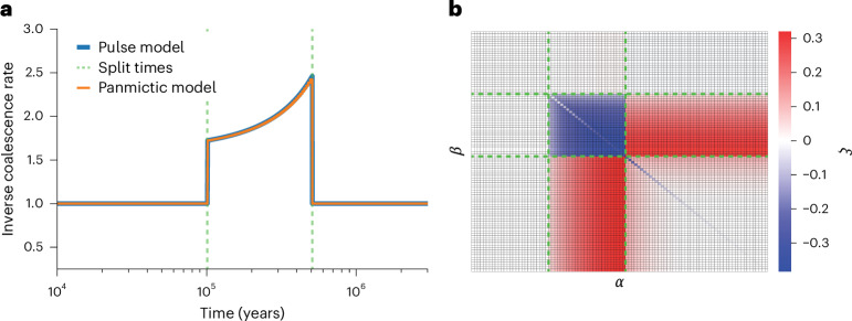
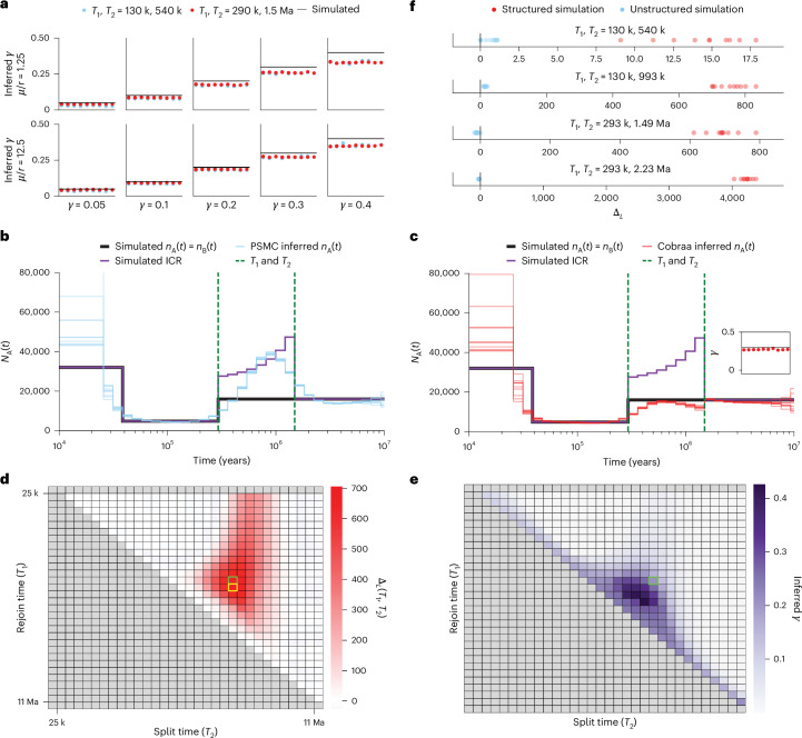
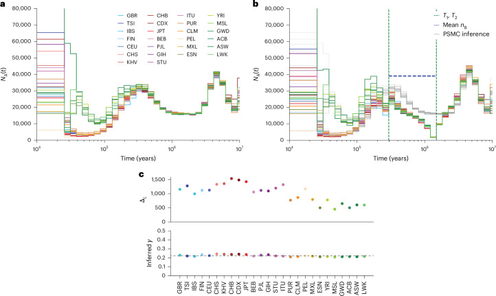
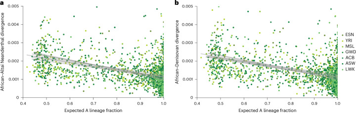
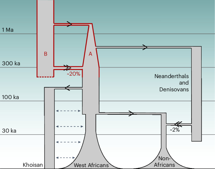
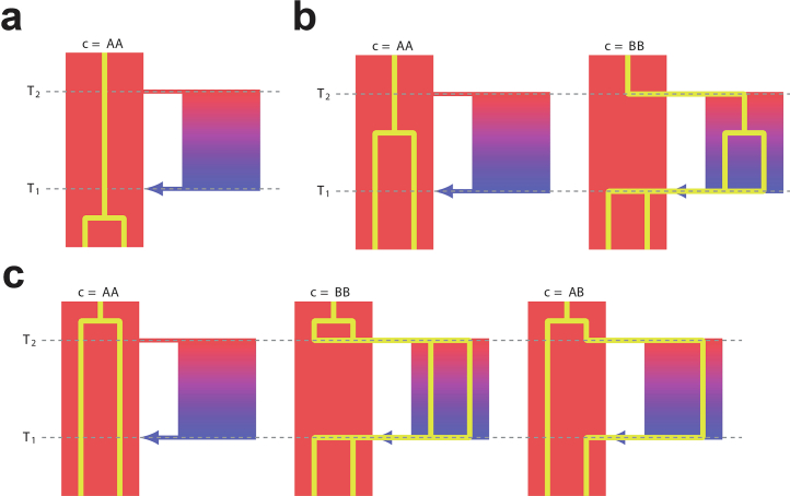
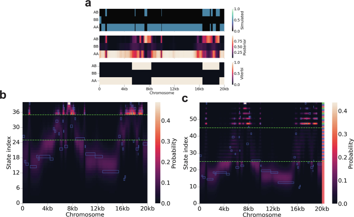
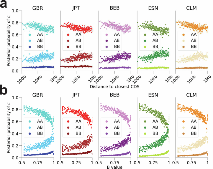
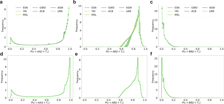
Understanding the history of admixture events and population size changes leading to modern humans is central to human evolutionary genetics. Here we introduce a coalescence-based hidden Markov model, cobraa, that explicitly represents an ancestral population split and rejoin, and demonstrate its application on simulated and real data across multiple species. Using cobraa, we present evidence for an extended period of structure in the history of all modern humans, in which two ancestral populations that diverged ~1.5 million years ago came together in an admixture event ~300 thousand years ago, in a ratio of ~80:20%. Immediately after their divergence, we detect a strong bottleneck in the major ancestral population. We inferred regions of the present-day genome derived from each ancestral population, finding that material from the minority correlates strongly with distance to coding sequence, suggesting it was deleterious against the majority background. Moreover, we found a strong correlation between regions of majority ancestry and human-Neanderthal or human-Denisovan divergence, suggesting the majority population was also ancestral to those archaic humans.

Fig. 1. The structured ancestry model used by cobraa.

a, Diagram of the structured model. Going forward in time, an ancestral population splits into two populations, A and B, at time T₂. These remain in isolation until time T₁ when there is an admixture event. b, We extend the SMC model to include the structure in a. We consider two sampled lineages from population A at t = 0. The consequences of ancestral recombination are partitioned into ten mutually exclusive cases, with an example from each illustrated. The gold lines indicate the two chromosomes sampled from the present at a particular locus, and the green line indicates the ‘floating’ lineage under the SMC model, which coalesces somewhere higher up on the tree in either population A or B.

Fig. 2. Difference in transition matrices for matched structured and unstructured models.

a, Matching coalescence rate profiles for a structured and unstructured model. The blue line indicates the theoretical inverse coalescence rate for the structured model, where populations A and B are of constant size, the split and admixture times are given by the vertical, dashed green lines and the admixture fraction is 30%. The orange line indicates an unstructured model with size changes that generate a coalescence rate equal exactly to the structured model. b, A visualization of ξ = (Q^U − Q^S)/Q^S, the relative difference between the transition matrices for the structured and unstructured models in a. Q^U and Q^S are row stochastic matrices, where Q(α∣β) describes the probability of transitioning from discretized time β to time α, conditional on recombination having occurred. The dashed green lines indicate the split and admixture times as in a.

Fig. 3. Ability of cobraa to infer parameters of a structured model.

a, Inferring the admixture fraction γ, when the population sizes and split/admixture times are fixed at their simulated value. The simulated model has constant size in populations A and B, μ = 1.25 × 10⁻⁸ (top) or μ = 1.25 × 10⁻⁷ (bottom), r = 1 × 10⁻⁸, and 3 Gb of sequence data for various values of γ and (T₁,T₂). Ten replicates of each are shown. b, PSMC inference of N_A(t), on a simulated structured model. The black line indicates simulated N_A(t), which is the same as simulated N_B(t). The green, dashed, vertical lines indicate the split and admixture times (T₁ = 300 ka and T₂ = 1.5 Ma, respectively) with γ = 30%, μ = 1.25 × 10⁻⁸, r = 1 × 10⁻⁸ and 3 Gb of sequence data. The purple line is the simulated ICR. c, Cobraa inference of N_A(t) for the same structured model. The inset shows the inferred admixture fraction. d, Using cobraa to search for T₁ and T₂ by iterating EM till convergence and recording the log-likelihood. The vertical axis represents the admixture time T₁, with values closer to the top indicating more recent times. The horizontal axis represents the split time T₂, with values more right indicating more ancient times. The simulated (T₁,T₂) pair is highlighted in the green cell, and the maximum-likelihood (T₁,T₂) pair is highlighted in yellow. e, Corresponding inference of γ for each pair (relative error is shown in Supplementary Fig. 4). f, Difference in model fits between cobraa and PSMC, ${\mathrm{\Delta }}_{\mathcal{L}}={\mathcal{L}}_S-{\mathcal{L}}_U$, for a structured simulation (red points) and an unstructured simulation (blue points), both of which have the same coalescence rate profile. The third panel corresponds to the inference as shown in b and c. ICR, inverse coalescence rate.

Fig. 4. Inference from PSMC and cobraa on 26 individuals from the 1000GP.

a, PSMC’s estimate of N_A(t). b, cobraa’s estimate of N_A(t), with the estimated split and admixture times (~290 ka and ~1.5 Ma, respectively) shown in vertical, dashed, green lines. For direct comparison, the PSMC inference from a is also plotted in gray. The mean inferred size of population B, ~39,200, is shown in the horizontal, dashed, blue line. c, Top, the difference between the log-likelihood from cobraa’s inference and PSMC’s inference, ${\mathrm{\Delta }}_{\mathcal{L}}$ for each population; bottom, cobraa’s inferred admixture fraction γ. Identifiers for samples selected are given in Supplementary Table 1, and full names corresponding to triplet codes for the populations are given in Supplementary Table 5.

Fig. 5. Relationship between human–archaic divergence and cobraa-path’s expected fraction of ancestry from the A lineage.

a, Divergence to the Altai Neanderthal sequence, plotted against the mean of P(c = AA) + P(c = AB)/2, calculated in windows of 10 kb and shown as points (subsampled for clarity) for each of seven African individuals. b, Corresponding plot for divergence to the Denisovan sequence. As confidence in a region being assigned to the A lineage increases, both human–Neanderthal and human–Denisovan divergence decreases. This suggests that Neanderthals and Denisovans derive from population A. The gray lines show a linear line of best fit for each population.

Fig. 6. A simplified model of human demographic history, as inferred by cobraa.

A simplified model of human demographic history showing deep population structure ~1.5 Ma to ~300 ka ago shared by all present-day humans, as inferred by cobraa (red). Arrows indicate the direction of gene flow, with admixture events (double arrows) labeled by their percentage genetic contribution to the recipient population. Of the two ancestral branches A and B, A represents 80% of subsequent ancestry and features a sharp bottleneck immediately after its founding. Dashed arrows between Khoisan and other African populations reflect the fact that this divergence, the deepest among present-day human populations, has involved ongoing or intermittent gene flow^,,. The y axis represents time in years before the present.

Extended Data Fig. 1. Heterozygosity estimates for the 26 individuals from distinct populations in the 1000 Genomes Project.

The scaled mutation rate θ = 4Nμ per population in the 1000 Genomes Project, using Waterson’s estimator. The dashed, horizontal line indicates the mean. See Supplementary Table 1 for full information.

Extended Data Fig. 2. Differences in log-likelihood between various structured models and the unstructured model.

(a) The log-likelihood difference (${\mathrm{\Delta }}_{\mathcal{L}}={\mathcal{L}}_S-{\mathcal{L}}_U$) between cobraa and PSMC, for all given pairings of T₁ and T₂ for each population (ACB excluded). Each algorithm was run until convergence, defined as the change in $\mathcal{L}$ between subsequent iterations of the expectation-maximisation (EM) algorithm being less than one. Red indicates a positive difference, blue negative, and white zero. Each population is shown on its own scale. The green highlighted cell indicates the composite maximum likelihood (CML) estimate and the yellow highlighted cell indicates the maximum likelihood estimate per population. Higher on the y-axis indicates more recent T₁, and leftmost on the x-axis indicates more recent T₂. (b) A diagram indicating the corresponding time interval boundaries associated with each cell in a.

Extended Data Fig. 3. The inferred size of population B, for 26 individuals from the 1000 Genomes Project.

(a) Inference of N_A(t) from cobraa on 26 populations from the 1000 Genomes project, with the inferred size of the ghost population N_B(t) shown in the horizontal dashed lines. When optimizing we enforced that N_B(t) must be constant due to identifiability problems. (b) Fixing the inferred N_A(t), γ, T₁, T₂, and ρ as shown in a, we compute the likelihood of the data with varying values of N_B, for each population. The plot shows the difference between this model (${\mathcal{L}}_S\left(N_B\right)$) and the unstructured model (${\mathcal{L}}_U$) in Fig. 4a, ${\mathrm{\Delta }}_{\mathcal{L}}={\mathcal{L}}_S\left(N_B\right)-{\mathcal{L}}_U$. The circles on each line represent the maximum likelihood estimate.

Extended Data Fig. 4. Diagram of the cobraa-path model.

A diagram of the possible ancestral lineage paths, c, as explicitly modeled in cobraa-path. (a) If the coalescence time was more recent than the admixture event (T₁), the only possibility is that the lineages coalesce in population A, which we denote as c = AA. (b) If the coalescence time was in the structured period, between T₁ and T₂, then c = AA or c = BB. (c) If the coalescence time was more ancient than the split time, T₂, then c = AA, c = BB or c = AB.

Extended Data Fig. 5. Posterior decoding from cobraa and cobraa-path, on simulated data.

We can decode the HMM of cobraa-path to infer the admixed regions of the genome (that is parts of the genome where the ancestral lineage pair went through AB or BB). The top panel of a shows the simulated lineage path across the genome, where the x-axis indicates the chromosomal position and the y-axis the ancestral lineage path. A structured model was simulated with μ/r = 1.25, 40% admixture, and constant population sizes. Using the simulated structured parameters, the middle panel shows the marginal posterior probability of each lineage path (from the forward/backward algorithm), and the bottom shows the most likely lineage path (from the Viterbi algorithm). (b) The full cobraa decoding of the simulation (hidden states are discretized coalescence times), where the y-axis indicates the coalescence time with 0 being the present. The green, dashed, horizontal lines indicate the simulated split and admixture times. (c) The full cobraa-path decoding of the simulation (hidden states are discretized coalescence times and ancestral lineage path). The y-axis indicates not only the coalescence time but also the ancestral lineage path, which is indicated by the shading in the right-most column. Red indicates AA, blue BB, and green AB. In the structured period, a red-blue pair indicates the same coalescence time, and more anciently than the split time a red-blue-green triple indicates the same coalescence time. The simulated states through the model are shown by the highlighted blue cells, and the posterior probabilities are indicated by the shading of the heatmap, with cream representing total confidence and black indicating no confidence. The y-axis in (a) indicates the ancestral lineage path, and in b and c the coalescence time, with more ancient states at the top and more recent ones at the bottom. The horizontal, green, dashed lines in b and c indicate the split and admixture time.

Extended Data Fig. 6. Correlation between the probability of an admixed lineage path and functional genomic information.

Correlation between the inferred probability of an admixed lineage path (conditional on the coalescence time being older than the admixture event) and the distance to coding sequence (CDS) (a) or strength of B-value (b). To get the inferred probability of an admixed lineage path, we decode the HMM of cobraa-path with the parameters as inferred from cobraa (Fig. 4b,c), and marginalize out the coalescence times. The Spearman correlation coefficients for each population are shown in Supplementary Table 2.

Extended Data Fig. 7. Density of posterior probability assignments to lineage combinations AA, AB, and BB, for real and simulated data.

(a–c) The density of posterior probability assignments to lineage combinations AA, AB, and BB for African samples analyzed using cobraa-path under our best fit structured model. (d–f) Corresponding plots for 1Gb of simulated data using parameters from the ESN model. (b,e) Given that t > T₂ there is a high confidence in assignment to AB, because most AA pairs coalesce prior to the T₂ due to the bottleneck at the founding of population A. (c,f) Although there are some real BB lineages (prior probability = 0.04) we do not have power to confidently identify these.

Extended Data Fig. 8. cobraa analysis on other species.

Inference from cobraa on various species. (a–c) Shown are parti-coloured bat, (d–f) common dolphin, (g–i) gorilla and (j–l) chimpanzee. (a,d,g,j) The leftmost column indicates the difference between the structured model for various time pairings and the unstructured model, ${\mathrm{\Delta }}_{\mathcal{L}}={\mathcal{L}}_S\left(T_1,T_2\right)-{\mathcal{L}}_U$. (b,e,h,k) The middle column indicates the inferred admixture fraction γ from each time pairing. (c,f,i,l) The right column shows the inference of population size changes from PSMC and cobraa (the inferred size of N_B in (i) and (l) was 690 ka and 164 ka, respectively).

References

1. Reich, D. Who we are and how we got here: Ancient DNA and the new science of the human past. Oxford University Press, (2018).
1. Prüfer, K. et al. The complete genome sequence of a Neanderthal from the Altai Mountains. Nature505, 43–49 (2014). - PMC - PubMed
1. Green, R. E. et al. A draft sequence of the Neandertal genome. Science328, 710–722 (2010). - PMC - PubMed
1. Reich, D. et al. Genetic history of an archaic hominin group from Denisova Cave in Siberia. Nature468, 1053–1060 (2010). - PMC - PubMed
1. Meyer, M. et al. A high-coverage genome sequence from an archaic Denisovan individual. Science338, 222–226 (2012). - PMC - PubMed
LinkOut - more resources