Role of tristability in the robustness of the differentiation mechanism

Abstract

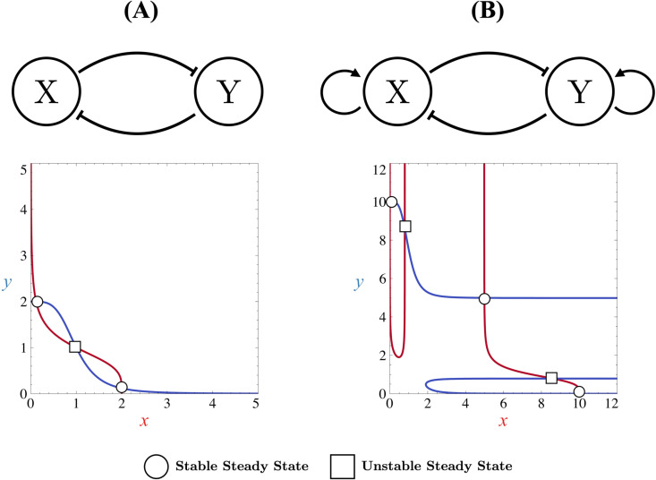
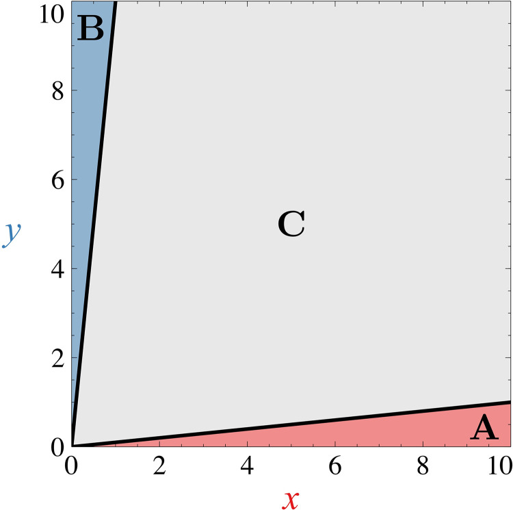
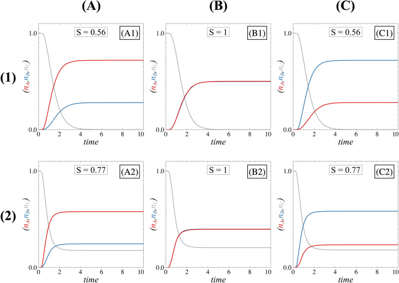
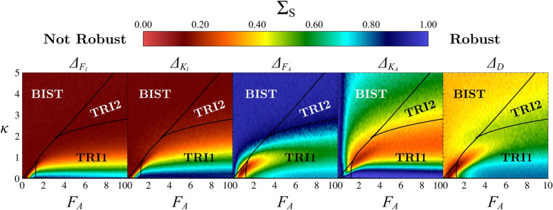
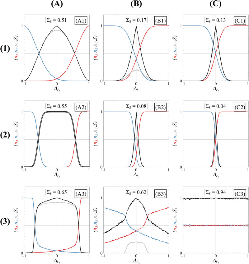
During cell differentiation, identical pluripotent cells undergo a specification process marked by changes in the expression of key genes, regulated by transcription factors that can inhibit the transcription of a competing gene or activate their own transcription. This specification is orchestrated by gene regulatory networks (GRNs), encompassing transcription factors, biochemical reactions, and signalling cascades. Mathematical models for these GRNs have been proposed in various contexts, to replicate observed robustness in differentiation properties. This includes reproducible proportions of differentiated cells with respect to parametric or stochastic noise and the avoidance of transitions between differentiated states. Understanding the GRN components controlling these features is crucial. Our study thoroughly explored an extended version of the Toggle Switch model with auto-activation loops. This model represents cells evolving from common progenitors in one out of two fates (A or B, bistable regime) or, additionally, remaining in their progenitor state (C, tristable regime). Such a differentiation into populations with three distinct cell fates is observed during blastocyst formation in mammals, where inner cell mass cells can remain in that state or differentiate into epiblast cells or primitive endoderm. Systematic analysis revealed that the existence of a stable non-differentiated state significantly impacts the GRN's robustness against parametric variations and stochastic noise. This state reduces the sensitivity of cell populations to parameters controlling key gene expression asymmetry and prevents cells from making transitions after acquiring a new identity. Stochastic noise enhances robustness by decreasing sensitivity to initial expression levels and helping the system escape from the non-differentiated state to differentiated cell fates, making the differentiation more efficient.

Fig 1. Topologies of simple GRNs governing cell differentiation mechanism.

Schematic representations of two GRNs: (A) a two-component mutually inhibitory feedback loop without autoactivation (Toggle Switch) and (B) the same loop with autoactivations (Self-activating Toggle Switch). In these circuits,  ⊣  arrows indicate gene inhibition in the transcription process, while  →  arrows represent gene activation in the transcription process. For each topology, the corresponding phase portrait is shown. Stable and unstable steady states are marked with circles and squares, respectively. Nullclines are included in the phase portraits, with the x-nullcline shown in red and the y-nuclline in blue.

Fig 2. Multistability domains for the GRN.

Stability diagrams for the system defined by Eqs (9) and (10) as a function of parameters $F_A$ and κ. Panels (A), (B), and (C) correspond to different values of inhibition force $F_I$ ((A) $F_I=2$, (B) $F_I=5$, (C) $F_I=10$). Each coloured zone represents a distinct stability domain as indicated.

Fig 3. Bistable behaviour.

Phase portrait depicting the dynamical system for different values of $F_I$ ($F_I=1$ (A), $F_I=2$ (B), $F_I=5$ (C)). In each panel, all ${\Delta }_i=0$, $F_A=0$ and $\kappa =0$. Corresponding manifolds for states A, B and C (in red, blue or grey, respectively) are also represented by solid lines (stable manifolds) or dashed lines (unstable manifolds). These manifolds are computed with the XPP-AUTO software. Different coloured zones in phase space illustrate basins of attraction, leading to trajectories ending in state A (red), state B (blue), or remaining non-differentiated in state C (grey).

Fig 4. Tristable behaviour.

Row (1) panels represent the phase portrait for different tristable regimes (Tristable I regime (column (A)), Tristable II regime (column (C)). The tristable I intermediate case is represented in panels (column (B)). Corresponding manifolds for states A, B and C (in red, blue or grey, respectively) are also represented by solid lines (stable manifolds) or dashed lines (unstable manifolds). 10 corresponding trajectories starting from ($x_0=0$, $y_0=0$) for each case leading to each state are shown in row (2) panels. Different coloured zones in the phase space illustrate basins of attraction, leading to trajectories ending in state A (red), state B (blue), or remaining non-differentiated in state C (grey). In each panel, all ${\Delta }_i=0$, $F_I=5$ and $F_A=5$. For column (A) panels, $\kappa =0.5$; for column (B) panels, $\kappa =1.2$; and for column (C) panels, $\kappa =2.5$.

Fig 5. Effect of asymmetries on bistability.

Bifurcation diagrams illustrating the influence of asymmetry parameters on the system (9)-(10). Panels (A), (B) and (C) represents variations in ${\Delta }_{FI}$, ${\Delta }_{KI}$, and ${\Delta }_D$, respectively, while $F_I$ is fixed at different values (2 (orange), 5 (purple) and 10 (green)). In each panel, all ${\Delta }_i=0$ except for the one that changes, $F_A=0$ and $\kappa =0$. Stable branches are depicted by continuous lines, while unstable branches are represented by dotted lines.

Fig 6. Effect of asymmetries on the bistable phase portrait.

Shift of steady states when asymmetry favours state A (column (A), $\Delta =0.1$) or state B (column (C), $\Delta =-0.1$) compared to the symmetric case (column (B), $\Delta =0$). Asymmetry applied through ${\Delta }_{FI}$, ${\Delta }_{KI}$ corresponds to rows (1) and (2) respectively. In each panel, $F_I=3$, $F_A=0$, $\kappa =0$ and all ${\Delta }_i=0$ except for the one that change. Corresponding manifolds for states A, B and C (in red, blue or grey, respectively) are also represented by solid lines (stable manifolds) or dashed lines (unstable manifolds). Different coloured zones in the phase space illustrate basins of attraction, leading to trajectories ending in state A (red), state B (blue), or remaining non-differentiated in state C (grey). In panels corresponding to an asymmetric case (A1, A2, C1, C2), both sets of steady states in the symmetric and asymmetric case are represented with a black or orange contour, respectively.

Fig 7. Effect of asymmetries on tristable phase portrait with a highly attractive non-differentiated state.

Shift of steady states when asymmetry favours state A (column (A), $\Delta =0.4$) or state B (column (C), $\Delta =-0.4$) compared to the symmetric case (column (B), $\Delta =0$). Asymmetry applied through ${\Delta }_{FI}$, ${\Delta }_{FA}$ corresponds to rows (1) and (2) respectively. In each panel, $F_I=5$, $F_A=5$, $\kappa =0.5$ and all ${\Delta }_i=0$ except for one that change. Corresponding manifolds for states A, B and C (in red, blue or grey, respectively) are represented by solid lines (stable manifolds) or dashed lines (unstable manifolds). Different coloured zones in the phase space illustrate basins of attraction, leading to trajectories ending in state A (red), state B (blue), or remaining non-differentiated in state C (grey). In panels corresponding to an asymmetric case (A1, C1, A2, C2), both sets of steady states in the symmetric and asymmetric case are represented with a black or orange contour, respectively.

Fig 8. Effect of asymmetries on tristable phase portrait with a poorly attractive non-differentiated state.

Shift of steady states when asymmetry favours the A state (column (A), $\Delta =0.4$) or the B state (column (C), $\Delta =-0.4$) compared to the symmetric case (column (B), $\Delta =0$). Asymmetry applied through ${\Delta }_{FI}$, ${\Delta }_{FA}$ corresponds to rows (1) and (2) respectively. In each panel, $F_I=5$, $F_A=5$, $\kappa =1.2$ and all ${\Delta }_i=0$ except for one that change. Corresponding manifolds for states A, B and C (in red, blue or grey, respectively) are represented by solid lines (stable manifolds) or dashed lines (unstable manifolds). Different coloured zones in the phase space illustrate basins of attraction, leading to trajectories ending in state A (red), state B (blue), or remaining non-differentiated in state C (grey). In panels corresponding to an asymmetric case (A1,C1,A2,C2), both sets of steady states in the symmetric and asymmetric case are represented with a black or orange contour, respectively).

Fig 9. Spatial coarse graining of phase space.

Black lines represent the different boundaries between each coarse-grained state and are given by Eqs (11) and (12). In this case, $F_I=0$. Trajectories that are in the red, blue or grey domains corresponds to A, B or C cells respectively.

Fig 10. Time evolutions of proportions.

Time evolutions of the proportions of trajectories occupying states A ($n_A$, red curve), B ($n_B$, blue curve), or C ($n_C$, grey curve). Column (A) panels and column (C) panels depict the time evolutions for an asymmetric GRN ($\Delta =0.1$, $\Delta =-0.1$, respectively) while column (B) panels stand for a symmetric, in both bistable (or tristable II) (row (1)) and tristable I (row (2)) scenarios. In all panels, $F_I=5$. For row (1) panels, $F_A=0$ and $\kappa =0$; for row (2) panels, $F_A=5$ and $\kappa =1.5$. For column (A) and (C) panels, the asymmetry is applied through $\Delta F_I$ which is equal to $0.1$ and $-0.1$, respectively. The system size Ω is equal to 10. Proportions were calculated as fractions of trajectories ending A, B or C domain defined by our coarse graining for 10.000 Gillespie simulations.

Fig 11. Robustness diagrams in parametric space.

Parametric space spanned by $F_A$ and κ for different types of asymmetries taken one by one. $F_I$ is fixed at 5, and the system size is $\Omega =10$ (other values of $F_I$ and Ω are provided in S3 Fig). The colour scale represents the ${\Sigma }_S$ value at the steady state which is the mean of S over the entire domain of possible values for only one given asymmetry $({\Delta }_i=-1$ to ${\Delta }_i=1$). Red zones (${\Sigma }_S\approx 0$) indicate less robust cases, while blue zones (${\Sigma }_S=1$) denote the most robust parametric regions with respect to the asymmetry which is considered. For each ($F_A,\kappa$), ${\Sigma }_S$ is computed at the steady state from 200 Gillespie simulations. The system is considered stationary after 20-time units. Stability domains are the same as in Fig 2. Simulations were performed in the parametric space with a discretization step of 0.1 for κ and $F_A$.

Fig 12. Impact of regime on asymmetry-dependent steady state proportions.

Proportions of A cells (red), B cells (blue), and non-differentiated C cells (grey) as a function of the asymmetry level ${\Delta }_{FI}$ (rows (1)-(2)) and ${\Delta }_{FA}$ (row (3)). Three different regimes are shown: the tristable I where C is highly attractive (column (A)), tristable I where C is poorly attractive (column (B)), and bistable or tristable II (column (C)). Black curves represent the symmetry measure, $S=1-\left|n_A-n_B\right|$, with spreads reflecting the ${\Sigma }_S$ value (noted in each panel). In all panels, $F_I=5$ and $F_A=5$ but the value of κ changes: column (A) panels use $\kappa =0.5$, column (B) panels use $\kappa =1.5$, and column (C) panels use $\kappa =5.0$. Rows (1)-(3) and row (2) correspond to system sizes $\Omega =10$ and $\Omega =100$, respectively. Proportions were calculated as fractions of trajectories ending in A, B or C domains defined by our coarse graining for 10.000 Gillespie simulations. The system is considered stationary after 20-time units.

Fig 13. Transitions between states for different scenario.

Each column (A), (B) or (C) indicates a different transition scenario: $A\rightleftarrows B$ (column (A)), A or $B\to C$ (column (B)), $C\to A$ or B (column (C)). Row (1) panels represents time evolution trajectories of x (red lines) and y (blue lines) concentrations. Row (2) panels display the steady state probability distributions as a function of macroscopic variables x and y. These distributions are computed from 10.000 simulations. Row (3) panels display kinetic potentials at the steady state as a function of the variable $x-y$. These potentials are calculated based on the corresponding steady-state probability distributions, obtained through the Gillespie algorithm over 100.000 simulations, which are then smoothed into continuous distributions using kernel density estimation. The system is considered stationary after 20-time units. Il all scenarios, $F_I=2$. For the first scenario ($A\rightleftarrows B$ column (A)), $F_A=0$ and $\kappa =0$; for the second scenario (A or $B\to C$, column (B)), $F_A=3$ and $\kappa =0.4$; and for the third scenario ($C\to A$ or B, column (C)), $F_A=3$, $\kappa =1.2$. For each case, the extensivity parameter $\Omega =10$.

Fig 14. Transition probability between A and B states.

Panels (A) and (B) display the transition probability $p_{ab}$ between states A and B in the parametric space $F_A,\kappa$ for different values of $F_I=2$ (panel A) and $F_I=5$ (panel B). The color scale indicates the values of $p_{AB}$ which is computed by taking the mean value of the number of occurrences where the trajectory crosses from one differentiated state domain to another for 200 Gillespie simulations. The time window during which the number of transitions is counted starts at steady state (20-time units) and ends after 500-time units in order to broadly evaluate the number of transitions observed. Stability domains (black solid lines) are the same as in Fig 2. The black arrow indicates a reduction of $p_{AB}$ even if the system remains bistable as explained in the main text. Simulations were performed in the parametric space with a discretization step of 0.1 for κ and $F_A$.

Fig 15. Transition between differentiated and non-differentiated states.

Panels (A) and (B) display the mean value of $\Delta n_C=n_C\left(t_s+\Delta t\right)-n_C\left(t_s\right)$ from 2000 Gillespie simulation in the parametric space $F_A,\kappa$ for different values of $F_I=2$ (panel A) and $F_I=5$ (panel B). The system is considered stationary after 20 times units ($t_S=20$) and each simulation stops at $t=1000$ (i.e., $\Delta t=980$). The extensivity parameter $\Omega =10$. Red and orange/yellow zones ($\Delta n_C>0$) signify transitions from the non-differentiated state to the differentiated states, while blue and dark green zones ($\Delta n_C<0$) signify transitions from the differentiated states to the non-differentiated state. Light green zones indicate no observed transitions in the system. Stability domains (black solid lines) are the same as in Fig 2. Simulations were performed in the parametric space with a discretization step of 0.1 for κ and $F_A$.

References

1. Zhou JX, Huang S. Understanding gene circuits at cell-fate branch points for rational cell reprogramming. Trends Genet. 2011;27(2):55–62. doi: 10.1016/j.tig.2010.11.002 - DOI - PubMed
1. Jia D, Jolly MK, Harrison W, Boareto M, Ben-Jacob E, Levine H. Operating principles of tristable circuits regulating cellular differentiation. Phys Biol. 2017;14(3):035007. doi: 10.1088/1478-3975/aa6f90 - DOI - PubMed
1. Huang S, Guo Y-P, May G, Enver T. Bifurcation dynamics in lineage-commitment in bipotent progenitor cells. Dev Biol. 2007;305(2):695–713. doi: 10.1016/j.ydbio.2007.02.036 - DOI - PubMed
1. Duff C, Smith-Miles K, Lopes L, Tian T. Mathematical modelling of stem cell differentiation: the PU.1-GATA-1 interaction. J Math Biol. 2012;64(3):449–68. doi: 10.1007/s00285-011-0419-3 - DOI - PubMed
1. Gardner TS, Cantor CR, Collins JJ. Construction of a genetic toggle switch in Escherichia coli. Nature. 2000;403(6767):339–42. doi: 10.1038/35002131 - DOI - PubMed
LinkOut - more resources