Gauge fixing for sequence-function relationships

Abstract

Quantitative models of sequence-function relationships are ubiquitous in computational biology, e.g., for modeling the DNA binding of transcription factors or the fitness landscapes of proteins. Interpreting these models, however, is complicated by the fact that the values of model parameters can often be changed without affecting model predictions. Before the values of model parameters can be meaningfully interpreted, one must remove these degrees of freedom (called "gauge freedoms" in physics) by imposing additional constraints (a process called "fixing the gauge"). However, strategies for fixing the gauge of sequence-function relationships have received little attention. Here we derive an analytically tractable family of gauges for a large class of sequence-function relationships. These gauges are derived in the context of models with all-order interactions, but an important subset of these gauges can be applied to diverse types of models, including additive models, pairwise-interaction models, and models with higher-order interactions. Many commonly used gauges are special cases of gauges within this family. We demonstrate the utility of this family of gauges by showing how different choices of gauge can be used both to explore complex activity landscapes and to reveal simplified models that are approximately correct within localized regions of sequence space. The results provide practical gauge-fixing strategies and demonstrate the utility of gauge-fixing for model exploration and interpretation.

Fig 1. Choice of gauge impacts model parameters.

(A–C) Parameters, expressed in three different gauges, for an additive model describing the (negative) binding energy of the E. coli transcription factor CRP to DNA. Model parameters are from [37]. In each panel, additive parameters ${\theta }_l^c$ are shown using both (top) a heat map and (bottom) a sequence logo [39]. The value of the constant parameter ${\theta }_0$ is also shown. (A) The zero-sum gauge, in which the additive parameters at each position sum to zero. (B) The wild-type gauge, in which the additive parameters at each position quantify activity differences with respect to a wild-type sequence, $s^{\text{wt}}$. The wild-type sequence used here (indicated by dots on the heat map) is the CRP binding site present at the E. coli lac promoter. (C) The maximum gauge, in which the additive parameters at each position quantify differences with respect to the optimal character at that position. Note that, while the value of each additive parameter ${\theta }_l^c$ varies between panels A-C, differences of the form ${\theta }_l^c–{\theta }_l^{c^{\prime }}$ are preserved.

Fig 2. Geometry of gauge spaces for additive one-hot models.

(A–C) Geometric representation of the gauge space Θ to which the additive parameters at each position l are restricted in the corresponding panel of Fig 1. Each of the four sequence features (${\theta }_l^A$, ${\theta }_l^C$, ${\theta }_l^G$, and ${\theta }_l^T$) corresponds to a different axis. Note that the two axes for ${\theta }_l^G$ and ${\theta }_l^T$ are shown as one axis to enable 3D visualization. Black and gray arrows respectively denote unit vectors pointing in the positive and negative directions along each axis. G indicates the space of gauge transformations.

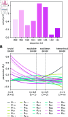
Fig 3. Binary landscape expressed in various parametric family gauges.

(A) Simulated random activity landscape for binary sequences of length L = 3. (B) Parameters of the all-order interaction model for the binary landscape as functions of η = λ/(1 + λ). Values of η corresponding to different named gauges are indicated. Note: because the uniform distribution is assumed in all these gauges, the hierarchical gauge is also the zero-sum gauge.

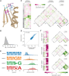
Fig 4. Landscape exploration using hierarchical gauges.

(A) NMR structure of GB1, with residues V39, D40, G41, and V54 shown (PDB: 3GB1, from [66]). (B) Distribution of log₂ enrichment relative to wild-type measured by [60] for nearly all 160,000 GB1 variants having mutations at positions 39, 40, 41, and 54. (C) Pairwise interaction model parameters inferred from the data of [60], expressed in the uniform hierarchical gauge (i.e., the zero-sum gauge). Boxes indicate parameters contributing to the wild-type sequence, VDGV. (D) Performance of pairwise-interaction model. Axes reflect log₂ enrichment values relative to wild-type. Each dot represents a randomly chosen variant GB1 protein assayed by [60]. For clarity, only 5,000 of the ∼160,000 assayed GB1 variants are shown. (E) Probability logos [39] for uniform, region 1, region 2, and region 3 sequence distributions. Distributions of pairwise interaction model predictions for each region are also shown. (F) Model parameters expressed in the region 1, region 2, and region 3 hierarchical gauges. Dots and tick marks indicate region-specific constraints. Probability densities (panels B and D) were estimated using DEFT [45]. Pairwise interaction model parameters were inferred by least-squares regression using MAVE-NN [39]. Regions 1, 2, and 3 were defined based on [64]. NMR: nuclear magnetic resonance. GB1: domain B1 of protein G.

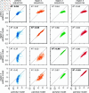
Fig 5. Model coarse-graining using hierarchical gauges.

Shown are data for 500 random 4 aa sequences generated using each of the four distributions listed in Fig 4E (i.e., uniform, region 1, region 2, and region 3). Vertical axes show log₂ enrichment (relative to wild-type) as predicted by additive models of GB1 derived by model truncation using region-specific zero-sum gauges (from Fig 4C and 4F). Horizontal axes show predictions of the full pairwise-interaction model. Diagonals indicate equality. GB1: domain B1 of protein G.

References

1. Kinney JB, McCandlish DM. Massively parallel assays and quantitative sequence-function relationships. Annu Rev Genomics Hum Genet. 2019;20:99–127. doi: 10.1146/annurev-genom-083118-014845 - DOI - PubMed
1. Weinberger ED. Fourier and Taylor series on fitness landscapes. Biol Cybern. 1991;65:321–30.
1. Stadler PF. Landscapes and their correlation functions. J Math Chem. 1996;20:1–45.
1. Weinreich DM, Lan Y, Wylie CS, Heckendorn RB. Should evolutionary geneticists worry about higher-order epistasis?. Curr Opin Genet Dev. 2013;23(6):700–7. doi: 10.1016/j.gde.2013.10.007 - DOI - PMC - PubMed
1. Poelwijk FJ, Krishna V, Ranganathan R. The context-dependence of mutations: a linkage of formalisms. PLoS Comput Biol 2016;12(6):e1004771. doi: 10.1371/journal.pcbi.1004771 - DOI - PMC - PubMed
LinkOut - more resources