The landscape of N6-methyladenosine in localized primary prostate cancer

Abstract

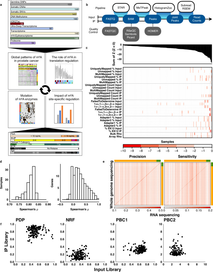
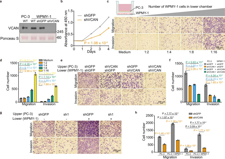
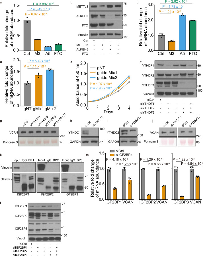
N⁶-methyladenosine (m⁶A), the most abundant internal RNA modification in humans, regulates most aspects of RNA processing. Prostate cancer is characterized by widespread transcriptomic dysregulation; therefore, we characterized the m⁶A landscape of 162 localized prostate tumors with matched DNA, RNA and protein profiling. m⁶A abundance varied dramatically across tumors, with global patterns emerging via complex germline-somatic cooperative regulation. Individual germline polymorphisms regulated m⁶A abundance, cooperating with somatic mutation of cancer driver genes and m⁶A regulators. The resulting complex patterns were associated with prognostic clinical features and established the biomarker potential of global and locus-specific m⁶A patterns. Tumor hypoxia dysregulates m⁶A profiles, bridging prior genomic and proteomic observations. Specific m⁶A sites, such as those in VCAN, drive disease aggression, associating with poor outcomes, tumor growth and metastasis. m⁶A dysregulation is thus associated with key events in the natural history of prostate cancer: germline risk, microenvironmental dysregulation, somatic mutation and metastasis.

Fig. 1. The m⁶A landscape of localized prostate cancer.

a, Top to bottom, bar plots. The number of MeTPeak peaks across samples ordered from greatest to smallest. The number of genomic rearrangements (GRs) identified in each sample. The number of single-nucleotide variants (SNVs) identified in each sample. The PGA as a proxy of the total CNAs for each sample. The Conti PRS calculated for each sample. Top heatmap shows the associated clinical covariates including ISUP Grade Group, anatomical T category, PSA, age, IDC/CA, biochemical relapse (BCR) and metastasis. Bottom heatmap, complementary molecular profiling data collected for each sample including germline polymorphisms in samples of European ancestry, somatic CNAs and simple somatic mutations, DNA methylome, H3K27ac, ultra-deep RNA-seq and proteomics. SSM, simple somatic mutation; N/A, not available. b–e, Exemplar plots for AR (the inset magnifies the region highlighted in yellow; b), MYC (c), TP53 (d) and PTEN (e). In the top polygon plots, the median IP (green) and input (purple) coverage (reads per kilobase per million mapped reads-normalized bigWig files) is represented using lines, while background colors represent the range of IP and input coverage across samples. Exons identified in GENCODE version 34 are annotated below in dark blue. Bottom heatmaps represent the distribution of IP and input coverage (log1p transformed) across samples (y axis), and darker colors correspond to greater read coverage. Samples are clustered using Euclidean distance and Ward’s minimum variance method with squared distances. chr, chromosome. f, Top bar plot, the number of peaks uniquely found in a given number of samples. Bottom scatterplot, the median adjusted m⁶A abundance of a joint peak (y axis) versus the number of samples in which the peak is identified (x axis). Colors indicate the deciles of the adjusted m⁶A abundance. Multiple joint peaks can be identified in a single gene, but the most prevalent and abundant peaks for a given gene are labeled where applicable. g, Distribution of the normalized mutual information (MI) for each data type pair. For visualization, values < 10⁻⁴ are shown as 10⁻⁴. Top heatmap indicates data type pair. Subsequent heatmaps show the number of genes with data available for each data type pair, numbers of genes for which mutual information is significant (Q < 0.1) and percentage of significant genes. Source data

Fig. 2. Molecular subtyping and clinical correlates of m⁶A.

a, Clustering of the top quartile of interquartile range (IQR)-ranked m⁶A peaks (n = 5,203) identified five patient subtypes and five m⁶A subtypes. Clinical covariates are shown to the right of the heatmap. Heatmap coloring indicates z-score-scaled peak intensities. b, Association between m⁶A patient subtypes and clinical features. Q values are from Pearson’s χ² test for categorical variables and a one-way ANOVA for continuous variables. c,d, Overlap of m⁶A patient clusters with pathologic tumor extent (pT) (c) and IDC/CA status (d). Patient clusters are indicated in rows, and clinical features are shown in columns. Row and column totals are depicted in the right and bottom heatmaps. Independence of clusters and clinical variables was assessed via Pearson’s χ² test (P value shown). The relative intensity of blue shading indicates the size of the group. e, Biochemical relapse rate across the five m⁶A patient subtypes. A Cox proportional hazards model was fit with P1 as the baseline group. Hazard ratios (HR) and P values are shown with confidence intervals in parentheses. f–h, Association between m⁶A patient subtypes and mutations in m⁶A regulators. f, Bar plot shows Q values from Pearson’s χ² test. ETS, E26 transformation-specific (ETS) transcription factor family members. g, Overlap of m⁶A patient clusters with presence of copy number gain of YTHDF1. h, Overlap of m⁶A patient clusters with presence of copy number gain of FANCA. Patient clusters are indicated in rows, and mutations are shown in columns. Row and column totals are depicted in the right and bottom heatmaps. Independence of clusters and mutations was assessed via Pearson’s χ² test (P value shown). The relative intensity of blue shading indicates the size of the group. i, BORCS6 m⁶A peak abundance varies by pISUP Grade Group. P value from one-way ANOVA is shown (n = 148). Box plots represent the median (center line) and upper and lower quartiles (box limits), and whiskers extend to the minimum and maximum values within 1.5× the IQR. j, NSD1 m⁶A peak abundance is greater with presence of IDC/CA. P value from two-sided U-test is shown; samples where IDC status was missing have been removed (n = 133). Box plots represent the median (center line) and upper and lower quartiles (box limits), and whiskers extend to the minimum and maximum values within 1.5× the IQR.

Fig. 3. Germline correlates of m⁶A in primary prostate cancer.

a, Allelic imbalance of reads at SNPs in annotated m⁶A sites in heterozygous samples in either the IP or input library. Allelic imbalance is evaluated using a paired t-test at a statistical threshold of Q < 0.1. Effect size (log₂ (fold change (FC))) is calculated with respect to the A allele. Effect size and direction are represented by the size and color of the disks, respectively. Statistical significance is represented by the background color. b, Distribution of P values in associations of m⁶A peak status with Conti PRS (t-test). c, m⁶A methylation of SRRM2 (peak 4) is associated with a lower Conti PRS (t-test). Box plots represent the median (center line) and upper and lower quartiles (box limits), and whiskers extend to the minimum and maximum values within 1.5× the IQR. n = 133. d, Significant prostate cancer risk SNP local m⁶A-QTLs identified using a linear additive model. Effect size (β) and direction are represented by the size and color of the disks, respectively. Statistical significance is represented by the background color. e,f, Two local risk SNP quantitative trait loci are depicted: the associations of genotype with m⁶A methylation for B3GAT1 (rs878987 | peak 13) (e) and RAB29 (rs708723 | peak 1) (f), respectively. Box plots represent the median (center line) and upper and lower quartiles (box limits), and whiskers extend to the minimum and maximum values within 1.5× the IQR. n = 133. g, Manhattan plot of genome-wide m⁶A-QTL analysis. Results from a linear additive model implemented in Matrix eQTL. Points representing the tag SNPs of m⁶A-QTLs where the gene has been annotated in the Cancer Gene Census or by Armenia et al., Fraser et al. and Quigley et al. are indicated with black squares, while the SNPs of significant (Q < 0.1) m⁶A-QTLs where the SNP has been annotated in RMVar or by Cotter et al. are indicated with black diamonds. Labeled black disks selectively identify top hits that fall into neither of the former categories. SLC9A3R2 (NHERF2). h, A genome-wide significant m⁶A-QTL: SNP rs4951018 with SLC45A3 m⁶A abundance. Box plots represent the median (center line) and upper and lower quartiles (box limits), and whiskers extend to the minimum and maximum values within 1.5× the IQR. n = 133.

Fig. 4. Tumor hypoxia is associated with widespread m⁶A modulation.

a, Hypoxia correlates with m⁶A peak abundance. Top bar plot indicates sample hypoxia score. Left–middle heatmaps show the corresponding z-scored m⁶A peak abundance per sample for peaks with a hypoxia correlation (Spearman’s correlation, Q < 0.05, 1,184 peaks). Peaks are clustered by abundance values, and the two largest resulting clusters are displayed in separate heatmaps. Right–middle heatmaps display m⁶A peak annotations. ‘RNA–hypoxia correlation’ indicates whether RNA abundance for the corresponding genes is also correlated with hypoxia. Hypoxia-correlated peaks are enriched for several biological pathways, and subsequent columns indicate whether each corresponding gene is tagged with each of the enriched pathway terms. Bottom heatmap shows z-scored RNA abundance for m⁶A writers, readers and erasers. Right bar plot shows P values for Spearman’s correlation between RNA abundance and hypoxia. Pol, polymerase. b, Patient m⁶A subtypes are associated with varying hypoxia levels. P value from one-way ANOVA. Box plots represent the median (center line) and upper and lower quartiles (box limits), and whiskers extend to the minimum and maximum values within 1.5× the IQR. n = 146. c,d, Associations between m⁶A abundance for an example peak on NSD1. Hypoxia (n = 146) (c), PGA (n = 148) (d). Plots annotated with results from Spearman’s correlation. e, Overlap between hypoxia-specific peaks in V16A and PC-3 cells. f,g, Patient hypoxia-associated peaks significantly overlap with hypoxia-specific peaks in prostate cancer cell lines. Contingency tables showing results from two-sided Fisher’s exact test for association between patient hypoxia-associated peaks and V16A (f) and PC-3 (g) hypoxia-specific peaks. The relative intensity of blue shading indicates the size of the group. OR, odds ratio. h, Correlation between tumor m⁶A abundance and hypoxia for a peak region in HNRNPLL. This peak shows a corroboratory hypoxia association in both V16A and PC-3 cell lines. Plots annotated with results from Spearman’s correlation (n = 146).

Fig. 5. Quantifying the biomarker potential of m⁶A sites.

a, m⁶A regulatory genes are frequently mutated. m⁶A enzyme-encoding genes are shown on the y axis, and patient samples are on the x axis. Top bar plot represents the number of mutations per sample, while the right bar plot shows the number of mutations in each m⁶A regulatory gene across samples. Central heatmaps display the mutations in each enzyme for each sample. b–d, Meta-analysis of six independent patient cohorts identifies mutations in m⁶A regulatory genes as predictive of patient biochemical recurrence. b, Left heatmap depicts m⁶A regulatory gene, mutation type and category of m⁶A regulatory action. Forest plot shows hazard ratios and 95% confidence intervals of each mutation on biochemical recurrence, and left bar plot indicates corresponding P values from a Cox model. The far right bar plot displays average sample mutation rate across the patient cohorts (protein, n = 54, m⁶A, n = 148; RNA, n = 92; gain or loss, n = 146). c,d, Gain of VIRMA (c) and gain of YTHDF3 (d) predict decreased biochemical recurrence-free rate. VIRMA gain, n = 22; loss, 191. YTHDF3 gain, n = 23; loss, 186. P values displayed are from Cox proportional hazards models. e–i, m⁶A provides complementary prognostic information in profiling prostate cancer driver genes. e, Left heatmap shows driver genes and molecular data type analyzed. Forest plot shows hazard ratio and 95% confidence intervals for biochemical recurrence, and the right bar plot indicates corresponding P values from a Cox model. f,g, Influence of m⁶A and copy loss on biochemical recurrence-free rate for tumor suppressors TP53 (f) and NKX3-1 (g). Kaplan–Meier survival curves show the results from median dichotomizing m⁶A abundance to create four patient groups, while inset forest plots show results from treating m⁶A as a continuous variable. P values displayed are from Cox proportional hazards models. h,i, Relative m⁶A abundance by biochemical recurrence status for TP53 (h) and NKX3-1 (i). Plots show copy number, z-scored RNA, m⁶A and protein abundance, and biochemical recurrence status at censoring time. Patients are depicted in columns and are ordered by biochemical recurrence status followed by m⁶A abundance. j,k, m⁶A peak status predicts biochemical recurrence for specific peak sites on INHBA, VCAN and ZFHX4. j, Patients are represented in columns. Top heatmap displays biochemical recurrence status at censoring time. Middle heatmap shows patient peak status (peak sites depicted in row labels). Right bar plot shows P values from a Cox model. k, Presence of a VCAN m⁶A peak increases risk of biochemical recurrence. VCAN peak, n = 23; no peak, 125. P values displayed are from Cox proportional hazards models.

Fig. 6. VCAN drives proliferation and progression in vitro and in vivo.

a, Kaplan–Meier survival curves showing biochemical recurrence stratified by VCAN mRNA abundance across five cohorts (Gerhauser, Ross-Adams, Taylor, TCGA-PRAD and International Cancer Genome Consortium (ICGC)-PRAD-CA (CA, Canada)), grouped by median abundance of VCAN mRNA. A Cox proportional hazards model was used to compare the hazard of biochemical recurrence between the groups. b, Kaplan–Meier survival curves showing biochemical recurrence stratified by VCAN average optical density from the tissue microarrays (TMA), grouped by median VCAN average optical density. A Cox proportional hazards model was used to compare the hazard of biochemical recurrence between the groups. c, Quantification of a migration and invasion assay after shRNA-mediated knockdown of VCAN in PC-3 cells. Data are represented as mean ± s.d. of three biological replicates. P values were calculated using one-way ANOVA with Dunnett’s multiple-comparisons test. d, Tumor growth of xenografts derived from injected PC-3 cells infected with shRNAs targeting VCAN or green fluorescent protein (GFP) as the control. Data are shown as mean ± s.e.m. of five biological replicates. P values are from one-way ANOVA with Dunnett’s multiple-comparisons test. e, Writing efficiency was assessed by m⁶A meRIP-quantitative PCR (qPCR) in PC-3 cells. SETD7 was introduced here as a negative control. Data are represented as mean ± s.d. of three biological replicates. P values are calculated using one-way ANOVA with Dunnett’s multiple-comparisons test. g, guide RNA; gNT, non-targeting guide RNA. f, VCAN protein abundance after dCasRx-METTL3-based m⁶A writing in PC-3 cells was detected by western blot. Ponceau S stain serves as the loading control. Numbers on the right indicate the positions of molecular mass (kDa) standards. g,h, Migration and invasion of PC-3 cells after writing by the dCasRx-METTL3-based RNA-editing system guided by VCAN mRNA-targeting guide RNA mixes. Representative images (g) and quantification (h, mean ± s.d. of three biological replicates; one-way ANOVA with Dunnett’s multiple-comparisons test) are shown. Scale bar, 200 μm. i, RIP–qPCR showing the physical association of VCAN mRNA with IGF2BPs in PC-3 cells. Data are represented as mean ± s.d. of three biological replicates. P values were calculated using an unpaired two-sided Student’s t-test. IgG, immunoglobulin G. j, Western blot showing VCAN protein abundance change after knocking down each IGF2BP protein (siIGF2BP1, siIGF2BP2 and siIGF2BP3) or all three IGF2BPs (siIGF2BP123) in PC-3 cells. Ponceau S stain serves as the loading control. Numbers on the right indicate the positions of molecular mass (kDa) standards. Ctrl, control. k, Graphical representation of VCAN regulation by m⁶A. Source data

Extended Data Fig. 1. Data Analysis & Quality Control.

a) The study workflow: we investigate the role of the post-transcriptional RNA modification m⁶A in primary prostate tumors by examining global m⁶A patterns, germline origins, clinical associations, microenvironmental associations and functional impact. This builds on previous molecular profiling studies of this primary prostate tumor cohort including 133 genotypes, 148 CNA and 143 somatic mutation profiles, 146 DNA methylation, 29 H3K27ac ChIP-seq, 92 ultra-deep RNA-sequencing and 54 proteomic profiles. b) Data processing pipeline for meRIP-sequencing. c) Quality control metrics derived from the output of STAR, RSeQC, cutadapt and correlation of the Input library with previous transcriptome profiling datasets^,. Top barplot: the sum of negative Z-scores for each sample. Bottom heatmap: metric by sample matrix where colors denote the magnitude of negative Z-scores. d) Left panel: sample-level correlation of transcript abundance in 92 samples common between Input libraries of this study and ultra-deep bulk RNA-seq from Chen et al. (Spearman’s ⍴). Right panel: gene-level correlation of transcript abundance in the same datasets (Spearman’s ⍴). e) Validation of sample identity by comparing germline variants identified in the Input libraries and Houlahan et al.. Both axes are ordered identically, first, by ancestry (covariate: orange represents European ancestry, green represents non-European ancestry) and then, by sample ID. Heatmap color represents precision (left) and sensitivity (right). Precision is calculated as the intersection of RNA-seq and WGS variants divided by all RNA-seq variants. Sensitivity is calculated as the intersection of RNA-seq and WGS variants divided by all WGS variants. f) Comparisons of the PCR Duplicate Proportion (PDP), the Non-Redundant Fraction (NRF) and the PCR Bottlenecking Coefficients 1 and 2 (PBC1/2) for each sample. The metric values of the IP library (y-axis) are compared to the metric values of the Input library (x-axis).

Extended Data Fig. 2. Peak Calling & Central Dogma Integration.

a) The distribution of peaks identified by exomePeak and MeTPeak. Each dot in the scatterplot represents a sample, histograms show the distribution of m⁶A methylated genes and peaks across samples. Bottom histogram shows the distribution of the number of peaks identified per gene. b) Spearman’s correlation of the number of peaks and the library size. The size of the disks corresponds to the magnitude of Spearman’s ⍴ and the background color indicate the P value (two-tailed test). c-d) The number of peaks called using three IP libraries when randomly subsampled to 50%, 25% 10% and 1% of the original reads for exomePeak (c) and MeTPeak (d). e) Comparing the coverage of MeTPeak and exomePeak peaks using the Simpson Index (intersection/smallest set, median = 94.80%) and the Jaccard Index (intersection/union, median = 53.01%) for each sample. Inner panel: Overlap by genomic coverage with previously identified peaks in the REPIC database. f) Distribution of peak density across a metagene as called by MeTPeak. Line shows the density of the peaks identified by HistogramZoo while the blue background shows the variation of peak density across individual samples. Bottom plot shows the distribution of peaks annotated across transcriptomic elements. g-j) Exemplar plots for MALAT1 (g), FOXA1 (h), RB1 (i) and NKX3-1 (j). The median IP (green) and Input (purple) coverage are represented using lines while background colors represent the range of IP and Input coverage across samples. Exons are annotated below in dark blue. Bottom heatmaps represent the distribution of IP and Input coverage (log1p-transformed) across samples. k) Relationship between the number of samples with an m⁶A peak at each gene and the corresponding gene-level RNA abundance. Box plots represent the median (center line) and upper and lower quartiles (box limits), and whiskers extend to the minimum and maximum values within 1.5x the IQR. l) Distribution of spearman’s correlation between m⁶A level and input abundance. m-n) Relationship between gene-level RNA and protein abundance correlation and (m) gene-level m⁶A abundance and (n) the number of samples with an m⁶A peak at each gene. Spearman’s correlation and corresponding P value displayed (n = 3,233).

Extended Data Fig. 3. Clinical Correlates of m⁶A.

a) m⁶A peak abundance correlates with patient clinical features. b) TAOK2 m⁶A peak abundance is correlated with age. Spearman’s correlation and corresponding P value displayed. c) Presence of IDC/CA co-occurs with greater patient peak number. P value is from a Student’s t-test (n = 133). Box plots represent the median (center line) and upper and lower quartiles (box limits), and whiskers extend to the minimum and maximum values within 1.5x the IQR. d) Association between patient peak number and patient clinical features. Dot size represents the indicated effect size (where applicable) and background color indicates P value. Spearman’s rank correlation was employed for PGA, age, and PSA, Mann Whitney U test was used for IDC status and pT, one-way ANOVA was used for analysis of ISUP Grade Group, and a Cox Proportional Hazards model was applied to analyse association between median-dichotomized sample peak number and biochemical recurrence. e) Association between patient peak number and mutations in prostate cancer driver genes. Samples are ranked by the number of peaks identified in descending order. Barplot indicates the statistical significance of each association, assessed via U-test.

Extended Data Fig. 4. Germline Correlates of m⁶A.

a) The overlap of m⁶A sites identified in RMVar and Cotter et al. 2021 with germline SNPs genotyped as described in Houlahan et al.. b) The distribution of allele frequencies of the A for SNPs/m⁶A sites in prostate cancer joint peaks (red) compared to the A for SNPs/m⁶A sites outside of joint peaks (white). c) The SNP rs2240912 is associated with biochemical recurrence (Q < 0.1; Cox Proportional Hazards model). d) The difference in Conti PRS relative to m⁶A peak status (PRS_Peak - PRS_{No Peak}) across peaks assessed using Student’s T test (two-sided). e-f) Left: The distribution of P values in associations (two-sided T test) between m⁶A peak status and Schumacher PRS (e) and PHS290 (f). Right: Volcano plots showing log₁₀ P values versus effect sizes (Δ PRS). g) The association between Conti PRS versus the number of MeTPeak peaks per sample using Spearman’s correlation analysis (two-sided). h-i) Left: distribution of P values in modelling associations between risk SNPs and local m⁶A peak methylation (h) and spatially-associated m⁶A peak methylation (i) Right: Volcano plots of P values versus effect sizes from additive linear models (β). Data from linear additive model. j) Histogram of the distance (bps) between the m⁶A-QTL and associated m⁶A peak. k) The identification of significant RNA, protein and clinical associations based on tag SNPs and gene pairs of m⁶A-QTLs. l) RNA and protein associations identified using m⁶A-QTL tag SNP-gene pairs. The disk sizes and color are indicative of the magnitude and direction of the β values of a linear additive model while the background color indicates the Q value. m-n) The associations of the SNP rs4951018 with SLC45A3 RNA (m) and protein abundance (n). Box plots represent the median (center line) and upper and lower quartiles (box limits), and whiskers extend to the minimum and maximum values within 1.5x the IQR. P values from linear additive model (n = 133). o) Top: tables showing associations between ISUP-associated alleles and ISUP Grade Group. Q values are derived from the global Χ² test. Bottom: tables showing associations between pairs of alleles.

Extended Data Fig. 5. Somatic Mutations Modulate the m⁶A Landscape.

a-b) Association of (a) copy number aberrations or (b) RNA abundance with 1) RNA or protein abundance of the corresponding gene, or total sample peak number (Student’s t-test, two-sided), 2) clinical features: ISUP Grade Group, IDC status, pathological T category (Pearson’s Χ² test, two-sided), PSA, and age (Student’s t-test, two-sided). Black background indicates Q value < 0.1, whilst dot size represents (a) effect size or (b) Spearman’s correlation. c) Association of mutations in m⁶A regulatory genes and prostate cancer driver events. P values from a hypergeometric test (one-sided for over-representation) are represented by the color of the background, whilst the size of the dot represents the difference between observed and expected co-occurring mutations. Covariate bars indicate mutation type and, if applicable, GISTIC peak the mutation is located within. d) Consensus clustering of 3,432 differentially methylated m⁶A peaks (k = 5) associated with driver mutations or mutations to m⁶A regulators (k = 5). For each mutation, colors in the main heatmap indicate the log₂ fold change in m⁶A level, and right barplot the number of m⁶A peaks significantly differentially m⁶A methylated, between samples with and without the corresponding mutation. MC: mutation cluster; DMPC: differentially-methylated peak cluster. e) Pathway enrichment analysis performed on genes with differential m⁶A abundance associated with mutations in m⁶A enzymes or prostate cancer drivers. Each node represents an enriched pathway term (from GO:BP or REACTOME ontologies). Node colors represent mutations from (d), with some pathways only enriched through joint consideration of all genes associated with a whole mutation cluster (indicated through ‘Contribution’ key). f) Forest plot showing the hazard ratio and 95% confidence intervals for presence of an m⁶A peak associated with biochemical recurrence, and left barplot indicates corresponding P values from a Cox Proportional Hazards model. g-h) Presence of a m⁶A peak on g) INHBA or h) ZFHX4, increases risk of biochemical recurrence. INHBA peak samples n = 6, ZFHX4 peak samples n = 9, total samples = 148. P values from a Cox Proportional Hazards model.

Extended Data Fig. 6. VCAN as a Candidate m6A Driver Event.

a) Correlations in RNA abundance of INHBA, VCAN, and ZFHX4 in the TCGA-PRAD and ICGC PRAD-CA cohorts. Dot size is Spearman’s correlation; background shading is P value. b) Comparison of the VCAN mRNA abundance between samples with and without peaks by the Input RNA-seq data. Samples with m⁶A peaks (n = 23) and without m⁶A peaks (n = 124) were derived from independent biological samples. The P value was calculated with two-sided Mann-Whitney U test between samples with and without m⁶A peaks on VCAN mRNA. The top and bottom of the box represent the 75th and 25th percentiles, respectively, with the line inside the box indicating the median. Whiskers extend to 1.5 times the interquartile range from the 25th and 75th percentiles. The fold change of peak mean TPM relative to no peak mean TPM is shown. c) Comparison of the VCAN abundance between samples with and without peaks by protein mass spectrometry data. Samples with m⁶A peaks (n = 15) and without m⁶A peaks (n = 39) were derived from independent biological samples. A two-sided Mann-Whitney U test was used to compare the difference between the two groups. The top and bottom of the box represent the 75th and 25th percentiles, respectively, with the line inside the box indicating the median. Whiskers extend to 1.5 times the interquartile range from the 25th and 75th percentiles. The fold change of peak mean value relative to no peak mean value is shown. d) m⁶A peak signals of VCAN transcripts from meRIP-seq libraries of several prostate cancer cell lines and patient samples with (CPCG0196) or without (CPCG0255) VCAN m⁶A peaks identified. The vertical red line indicates the location of the significant peak. e) Kaplan-Meier survival curves showing biochemical recurrence stratified by VCAN mRNA abundance in the Gerhauser, Ross-Adams, Taylor, TCGA-PRAD and ICGC-PRAD CA cohorts. A Cox Proportional Hazards model was used to compare the hazard of biochemical recurrence between the groups.

Extended Data Fig. 7. VCAN Drives Prostate Cancer Progression.

a-c) Knockdown efficiency of VCAN mRNA by shRNAs (a), protein abundance (b) and by siRNAs (c) in PC-3 cells. All other Western blots for VCAN in this study are treated by chABC by default. Ponceau S as the loading control. Numbers indicate the positions of molecular mass (kDa) standards. Data are represented as mean ± SD of three biological replicates. P values are calculated using one-way ANOVA with Dunnett’s multiple comparisons test. d) The representative images of the migration and invasion assay of PC-3 cells after shRNA-mediated knockdown of VCAN. The experiment was conducted using three biological replicates for each condition. The scale bar represents 200 μm. e) The growth curve after siRNA-mediated knockdown of VCAN in PC-3. Data are represented as mean ± SD of three biological replicates. P values are calculated using one-way ANOVA with Dunnett’s multiple comparisons test. f-g) The migration and invasion assay of PC-3 cells after siRNA-mediated knockdown of VCAN. The representative images (f), and the quantification (g). Data are represented as mean ± SD of three biological replicates. The scale bar represents 200 μm. h-i) The tumor weight (left) and the tumor size (right) of xenografts derived from injected PC-3 cells (h), and the extravasation ability of PC-3 (i) infected with shRNAs targeting VCAN or GFP as the control. Xenografts are shown as mean ± SEM of five biological replicates, and the extravasation data are presented as mean ± SD of biological replicates (shGFP, n = 9; VCAN sh1, n = 7; VCAN sh2, n = 6). P values are calculated using one-way ANOVA with Dunnett’s multiple comparisons test. j) The volcano plot showed the significantly up/down-regulated genes (average FC > log₂(1.5), adjusted P value < 0.05, two-sided) between shGFP and shKD VCAN groups in PC-3 mouse xenografts. Adjusted P values were calculated using the Benjamini-Hochberg method. Vertical dashed lines indicate -log₂(1.5) and log₂(1.5), respectively, and the horizontal one marks adjusted P = 0.05. k) Dotmap representing top 10 enriched pathways after shKD VCAN in PC-3 mouse xenograft tumors. Dot size indicates the odds ratio and background color the Q values. Source data

Extended Data Fig. 8. VCAN Regulates Tumor-Stromal Crosstalk.

a) Knockdown efficiency of VCAN by shRNA in WPMY-1 cells was detected by Western blot. Ponceau S stain serves as the loading control, and molecular mass (kDa) standards are indicated on the right. Additionally, a sample from PC-3 cells is included for relative quantification, demonstrating comparable levels of VCAN extracted from the same volume of culture medium collected from an equal number of cells. The experiment was conducted using three biological replicates for each condition. b) The growth curve after shRNA-mediated knockdown of VCAN in WPMY-1. Data are represented as mean ± SD of three biological replicates. P value is calculated using an unpaired two-sided Student’s T test. c-f) Migration and invasion analysis of indirect coculture of PC-3 and WPMY-1 cells. PC-3 cells (2 × 10⁴) were seeded into the upper chamber containing serum-free medium, while WPMY-1 cells were seeded in the lower chamber containing 10% fetal bovine serum at varying ratios (PC-3 to WPMY-1) ranging from 1:2 to 1:16 as indicated (c-d). PC-3 cells (5 × 10⁴) were seeded into the upper chamber containing serum-free medium, while WPMY-1 cells were seeded in the lower chamber containing 10% fetal bovine serum at a fixed ratio of 1:8 (PC-3 to WPMY-1) (e-f). Representative images (c, e) and quantification (d, f, mean ± SD of three biological replicates; one-way ANOVA with Dunnett’s multiple comparisons test) are presented. The scale bar represents 200 μm. g-h) PC-3 cells with VCAN knockdown (shVCAN) or control (shGFP) were cultured either with or without WPMY-1 cells. In the coculture condition, WPMY-1 cells were seeded in the lower chamber at a ratio of 1:8 (PC-3 to WPMY-1) in medium containing 10% fetal bovine serum (FBS); in the monoculture condition, the lower chamber contained only medium with 10% FBS. Representative images (g) and quantification (h, mean ± SD of three biological replicates; two-sided Student’s t-test) are presented. The treatments (knockdown) for each group are indicated in the figure. The scale bar represents 200 μm. Source data

Extended Data Fig. 9. m⁶A Stabilizes VCAN mRNA and Promotes its Translation.

a-b) Knockdown efficiencies of the m⁶A regulators by shRNAs in PC-3 at RNA (a, Data are represented as mean ± SD of three biological replicates. P values are calculated using unpaired two-sided T test.) and protein level (b, Numbers indicate the positions of molecular mass (kDa) standards). c) Relative abundance of VCAN mRNA after knockdown m⁶A regulators in PC-3 cells. Ctrl:shRNA targets GFP, M3:METTL3, A5:ALKBH5. Data are represented as mean ± SD of three biological replicates; P values, unpaired Student’s T test. d-e) The VCAN mRNA abundance (d) and growth curve (e) of PC-3 cells after writing by VCAN mRNA-targeting guide RNA mixes. Data are represented as mean ± SD of three biological replicates. P values, one-way ANOVA with Dunnett’s multiple comparisons test. f-g) Knockdown efficiencies of YTHDFs (f) and corresponding VCAN protein abundance change (g) in PC-3 cells infected with siRNAs against each YTHDF were assessed by western blot. Numbers indicate the positions of molecular mass (kDa) standards. h-i) Knockdown efficiencies of YTHDC1 (h) and YTHDC2 (i) in PC-3 cells infected with siRNAs against each YTHDC were assessed by western blot. Vinculin was used as a loading control. Numbers on the right indicate the positions of molecular mass (kDa) standards. j) Western blot showing VCAN protein abundance change after knocking down YTHDC1 and YTHDC2 in PC-3 cells. Ponceau S stain serves as the loading control. Numbers on the right indicate the positions of molecular mass (kDa) standards. k) RIP efficiencies of the IGF2BP proteins were evaluated by western blot. Vinculin was included as negative control of the IPs. Numbers on the right indicate the positions of molecular mass (kDa) standards. l) Knockdown efficiencies of IGF2BPs in PC-3 cells infected with siRNAs against each IGF2BP were assessed by western blot. Vinculin was used as a loading control. Numbers on the right indicate the positions of molecular mass (kDa) standards. m) Relative VCAN mRNA abundance after siRNA-mediated knockdown of IGF2BPs in PC-3 cells. Data are represented as mean ± SD of three biological replicates. P values are from unpaired T test. Source data

Extended Data Fig. 10. m⁶A Regulates VCAN Expression via IGF2BPs.

a) Cell proliferation after siRNA-mediated knockdown of IGF2BPs in PC-3 cells. Data are represented as mean ± SD of three biological replicates. P values are calculated using one-way ANOVA with Dunnett’s multiple comparisons test. b-c) Migration and invasion of PC-3 cells after siRNA-mediated knockdown of IGF2BPs in PC-3 cells. P values are calculated using one-way ANOVA with Dunnett’s multiple comparisons test. The representative images (b), and the quantification (c). Data are represented as mean ± SD of three biological replicates. The scale bar represents 200 μm. d) Ribosome profiling analysis of sample fractions. The graph illustrates ribosome profiling, with the intensity of the signal (voltage) plotted on the y-axis and sample fractions collected on the x-axis. The fractions are grouped based on the presence of polysomes, with polysome and polysome-free fractions distinguished and labeled accordingly on the graph. e) Relative enrichment of VCAN, GAPDH, and U6 in the polysome-free and polysome-associated fractions of PC-3 cells were measured by qPCR. GAPDH and U6 were employed as controls. Data are represented as mean ± SD of three biological replicates. P values are calculated using an unpaired two-sided Student’s T test. f) VCAN protein abundance after dCasRx-METTL3-based m⁶A writing with or without knocking down of IGF2BP2 was detected by western blot. Ponceau S stain serves as the loading control. Numbers on the right indicate the positions of molecular mass (kDa) standards. Source data

References

1. Hanahan, D. & Weinberg, R. A. The hallmarks of cancer. Cell100, 57–70 (2000). - PubMed
1. Sinha, A. et al. The proteogenomic landscape of curable prostate cancer. Cancer Cell35, 414–427 (2019). - PMC - PubMed
1. Liu, J. et al. An integrated TCGA pan-cancer clinical data resource to drive high-quality survival outcome analytics. Cell173, 400–416 (2018). - PMC - PubMed
1. Huang, H., Weng, H. & Chen, J. m6A modification in coding and non-coding RNAs: roles and therapeutic implications in cancer. Cancer Cell37, 270–288 (2020). - PMC - PubMed
1. Zhao, B. S., Roundtree, I. A. & He, C. Post-transcriptional gene regulation by mRNA modifications. Nat. Rev. Mol. Cell Biol.18, 31–42 (2017). - PMC - PubMed
LinkOut - more resources