DELTA: a method for brain-wide measurement of synaptic protein turnover reveals localized plasticity during learning

Abstract

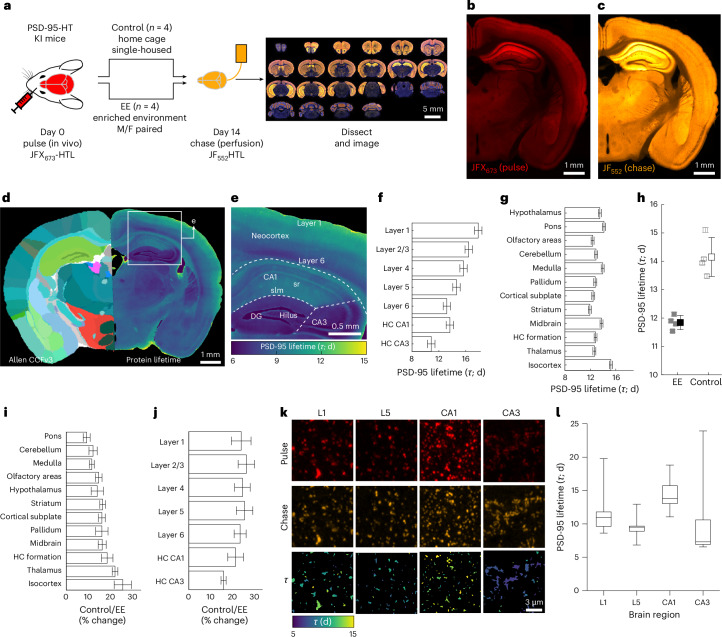
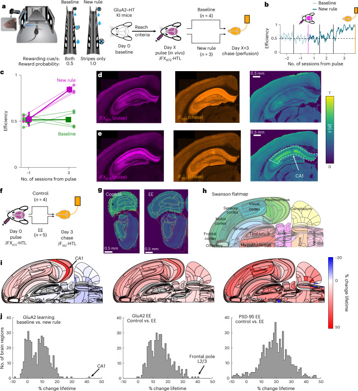
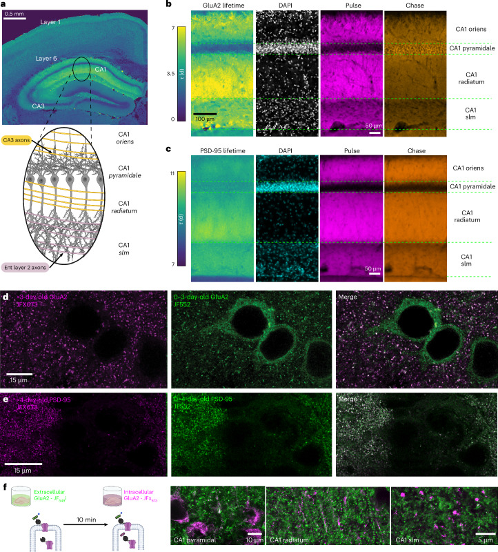
Synaptic plasticity alters neuronal connections in response to experience, which is thought to underlie learning and memory. However, the loci of learning-related synaptic plasticity, and the degree to which plasticity is localized or distributed, remain largely unknown. Here we describe a new method, DELTA, for mapping brain-wide changes in synaptic protein turnover with single-synapse resolution, based on Janelia Fluor dyes and HaloTag knock-in mice. During associative learning, the turnover of the ionotropic glutamate receptor subunit GluA2, an indicator of synaptic plasticity, was enhanced in several brain regions, most markedly hippocampal area CA1. More broadly distributed increases in the turnover of synaptic proteins were observed in response to environmental enrichment. In CA1, GluA2 stability was regulated in an input-specific manner, with more turnover in layers containing input from CA3 compared to entorhinal cortex. DELTA will facilitate exploration of the molecular and circuit basis of learning and memory and other forms of plasticity at scales ranging from single synapses to the entire brain.

Fig. 1. Measurement of protein turnover in vivo.

a, DELTA measures protein lifetime by sequential HTL dye capture using a HT-modified protein. (i) Before the injection of the first dye ligand (pulse), all proteins are unlabeled (gray line in graph). (ii) After injection of the pulse dye ligand (dashed green line), all proteins are labeled with the pulse dye ligand (solid green line, pulse). (iii) During the pulse–chase interval, some proteins degrade, and others are synthesized but are unlabeled. (iv) Injection of a spectrally separate chase dye ligand (dashed magenta line) binds the newly synthesized protein (solid magenta line, chase). The gray shaded area indicates where excess dye ligand delays the onset of turnover measurement, leading to a pulse overestimation error (Supplementary Text). b, The estimated lifetime error (color) as a function of dye-protein ratio (y axis) and true protein lifetime (x axis). Undersaturation (<1 dye ligand–protein ratio) causes worse errors than dye ligand excess and longer-lived proteins are estimated more accurately than short-lived ones. c,d, Turnover measurement of the nuclear protein MeCP2–HT in a knock-in (KI) mouse model. c, Experimental design: Three HTL dyes were used to measure multiple protein turnover intervals. After perfusion and dissection, coronal sections were labeled with DAPI and fluorescent antibodies to identify different cell types. d, Example field-of-view images showing the JF dyes with NeuN and DAPI for identification of neuronal nuclei. After segmentation of NeuN-positive nuclei, segmented nuclei were colored by lifetime using the sum of the two in vivo injections as the pulse (fraction pulse = (JF₆₆₉ + JF₅₅₂)/(JF₆₆₉ + JF₅₅₂ + JF₆₀₈)). e, Example coronal sections from two animals. Left and middle: images show the consistency of the lifetime estimates for aligned anteroposterior sections. Right: image shows the longer lifetime in the cerebellum (compared to middle and left images). f, MeCP2–HT neuronal nuclei lifetime (bootstrap of means from five animals and three intervals where the line is the median, boxes denote the 25th–75th percentiles and whiskers mark the 0.5th–99.5th percentiles) across CCF-aligned brain regions. a.u., arbitrary units.

Fig. 2. PSD-95 turnover depends on experience.

a, Experimental design for turnover measurement in a PSD-95–HT knock-in mouse. b–e, Example coronal sections showing the pulse (b), chase (c) and calculated lifetime aligned to the Allen CCFv3 (d and e). Note the lifetime gradient that separates the CA1 stratum radiatum (sr) and stratum lacunosum moleculare (slm; long lifetime) from dentate gyrus (DG) and hilus (all shorter lifetimes). f, Average ± s.e. lifetimes of control animals (n = 4). Cortical layers and subfields of the hippocampus (HC) were significantly different (mixed-effects linear model with layers as fixed effects (means: 10.0–16.5 days, s.e.: ~0.5, all P < 0.0001) and animal ID as a random effect (mean, 1.42 days; residual error, 1.39 days)). All mixed-effects models are double sided and without multiple-comparison corrections. g, Average ± s.e. lifetimes for 12 large brain regions were also significantly different in control mice (n = 4; mixed-effects linear model with brain regions as fixed effects (means: 11.9–15.2 days, s.e.: ~0.23, all P < 0.0001); animal ID as a random effect (mean: 0.46 days); residual error: 1.8 days). h, Average ± s.e. lifetimes of four mice under EE and four mice under control conditions. EE increased protein turnover and shortened the average lifetime of PSD-95–HT. Individual animals in gray (EE: 11.8 ± 0.2 days, n = 4; control: 14.2 ± 0.7 days, n = 4; two-sided Wilcoxon rank-sum test W = 26, P = 0.0286). i, Percentage change ± s.e. in control versus EE animals for 12 different brain regions; Mixed-effects linear model for each brain region with group assignment as fixed effects and animal as a random effect. j, Same as i for cortical layers and HC subfields. k, Example images using Airyscan imaging of ExM tissue (maximum projection of five z-planes, 0.3 μm apart) from layer 1, HC CA1 subfield and basal dendrites of CA3 showing both pulse, chase and lifetime (τ). l, Quantification of segmented single-synapse turnover (median lifetime in days; L1, 10.97; L5, 9.5; CA1, 13.78; CA3, 7.32). Boxes show the interquartile range and whiskers mark the 5th and 95th percentiles.

Fig. 3. Learning-induced GluA2 turnover is more localized than following environmental enrichment.

a, Turnover measurement in a GluA2–HT knock-in mouse during learning of a new behavioral rule (new rule). b, Example experiment showing efficiency (number of rewards per number of cues licked) across five daily sessions. Turnover was assessed by pulse dye ligand (JFX₆₇₃-HTL) injection before new-rule and chase dye ligand (JF₅₅₂-HTL) perfusion after the final session. c, Behavioral efficiency comparison between baseline (green, unchanged) and new-rule (magenta, improved) groups (n = 7). d,e, Coronal sections showing pulse (magenta), chase (orange) and calculated GluA2–HT lifetime (fast turnover, green and blue; slower turnover, yellow) for new-rule (d) and baseline (e) conditions, highlighting CA1 differences. Example from (c) n = 7 animals. f, Experimental design for turnover measurement of GluA2–HT modulated by environmental enrichment (EE). g, Example coronal sections from control mice and after EE. A black asterisk indicates the lower lifetime of GluA2–HT in frontal cortical regions. Example from n = 9 animals. Color scale is the same as in d. h, Swanson flatmap representation of mouse brain regions. Different colors represent different brain regions. i, Left: percentage change in GluA2–HT lifetime in baseline versus new rule. The largest effect is in CA1 (arrow). Middle: control versus EE groups. The largest effect is in the frontal pole (arrow). Right: percentage change in PSD-95–HT lifetime in control versus EE groups. j, Distribution of turnover changes across conditions. GluA2 learning (n = 442, median = 7.5%, 59.5% of brain regions with >5% change); GluA2 EE (n = 442, median = 14.3%, 94.8% >5%); PSD-95 EE (n = 580, median = 19.2%, 95.3% > 5%).

Fig. 4. Subcellular regulation of synaptic protein turnover.

a, Top: image of GluA2–HT lifetime in a coronal section. Bottom: schematic of the orientation of pyramidal cells in CA1 (gray) with inputs from CA3 (yellow) and entorhinal cortex (pink). Similar lifetime gradients were observed in all animals regardless of condition (n = 16). b, Lifetimes are low in the soma (stratum pyramidale), and increase in the proximal dendrites in stratum oriens and radiatum and decrease in the stratum lacunosum moleculare, implying subcellular control of synaptic protein turnover. c, Same as b for PSD-95–HT, showing similar turnover trends. d,e, Differences between GluA2–HT (d) and PSD-95–HT (e) in subcellular localization of newly synthesized protein. Whereas >3-day-old protein (magenta; left images) is mostly synaptically localized in both GluA2–HT (d) and PSD-95–HT (e), newly synthesized GluA2 (green; middle image in d) is enriched around the soma (in the cytosol while excluded from the nucleus; Supplementary Movie 2), but PSD-95–HT is not (green; middle image in e). Merged view in the right images. Similar gradients were observed in all animals regardless of condition (GluA2–HT, n = 16; PSD-95–HT, n = 8). f, Left: illustration of live slice experiment that separates extracellular and intracellular pools of GluA2–HT. The extracellular pool is first labeled with a cell-impermeable dye ligand (JF₅₄₉i-HTL, green) followed by labeling with a cell-permeable dye ligand (JFX₆₇₃-HTL, magenta). Both pools are seen in somata (first image) and both stratum radiatum and stratum lacunosum moleculare dendrites (second and third images; four brain slices).

Extended Data Fig. 1. HaloTag ligand dyes are cleared from the brain within hours.

a, Experimental procedure to measure dye-ligand clearance. The rise in fluorescence is not captured, as the animal is not imaged during the injection. b, Example images for a JF₆₆₉-HTL injection. The blue circle represents the region for which fluorescence was quantified in (c). Scale, 2 mm. c, Linear (left) and log (right) fluorescence (peak normalized and baseline subtracted) as JF₆₆₉-HTL is cleared from the brain. Double exponential fit in red; τ₁ and τ₂ are in minutes. d, Similar data for 12 experiments with 3 dyes (JF₅₂₅-HTL in green, JF₅₅₂-HTL in red, and JF₆₆₉-HTL in magenta). The black trace is a binned average, with standard error for all 12 experiments. The numbers in (d) represent the mean ± standard error of double exponential fits for the 12 experiments.

Extended Data Fig. 2. Modeling pulse-chase experiments in vivo, constrained by dye-ligand clearance measurements.

a, Model compartments, molecules, and reactions for modeling protein turnover measurements. A pulse or chase dye-ligand is added to the cytosol compartment and subsequently: (1) cleared; (2) can move to a lipid compartment (representing the slow dye-ligand clearance component); or (3) irreversibly binds to the protein-HT. Here, the protein synthesis rate is equal to its degradation rate, with dye-bound proteins degrading at the same rate. This maintains total protein amount constant regardless of dye-ligand binding. See Supplementary Text for more information. b, Fitting of the dye-ligand clearance data (Extended Data Fig. 1) to generate model variants. Twelve experiments (data in blue circles) and the fitted response (blue lines) are shown. The parameters fit were dye-ligand clearance rate, cytosol-to-lipid rate constant, and volume of the lipid compartment. The cytosol compartment was fixed to having a volume of 1 ml. c-e, Example model simulations with a selection of 7 HT-protein mean lifetimes (c: 10-640 h; Legend as in Fig. 1a). The correlation between estimated and true protein lifetime is excellent (d). The mean error (e, top) decreases with increasing lifetime, whereas the standard error between model variants (simulating variability in dye-ligand clearance) peaks around the mean dye-ligand clearance rate (e, bottom). f, Simulation of error in the lifetime estimate as a function of the pulse-chase interval (∆T). The error (blue line) decreases faster than the Pulse concentration (black line). This shows that the error with DELTA is dominated by dye-ligand clearance, with overall low error rates. g, Error in lifetime estimation using pulse-only measurements, given ideal dye-ligand injection delivery. Here, variability of the measurement across animals (CV y-axis) could be countered only by averaging across animals (number of animals x-axis). Error rates (color-coded) are higher than in DELTA, where the chase dye-ligand and the Fraction Pulse calculation normalizes for inter-animal variability under ideal dye-ligand injection conditions. h, Modeling to compare errors due to shot noise with DELTA (left panel) vs. pulse-only labeling (right panel). In both cases three measurement times (white dashed lines) were used to estimate a known decay (x-axis: 2-200 days). Increasing the signal to background ratio (y- axis) and adding a chase dye-ligand (as in DELTA; left panel) reduced shot-noise induced errors. i, Modeling the effects of a change in total protein on the error in lifetime estimation (% error in colormap) as a function of % change in protein levels (x-axis) and the measured fraction pulse (y-axis). Error increases with longer intervals (smaller fraction pulse) and larger changes in protein.

Extended Data Fig. 3. JF₅₅₂ and JF₆₆₉ are bioavailable in the brain.

a, Experimental procedures for dye-ligand screening in vivo. b, Example coronal sections imaged 4 weeks after infection with an AAV expressing GFP-HT. GFP fluorescence (left panel), fluorescence of JF₆₆₉-HTL injected in vivo (Pulse; middle panel), and fluorescence of JF₅₈₅-HTL fluorescence applied during perfusion (Chase; right panel). Scale bars, 200 µm. c, Example cell (square in b, left panel) overlaid with the mask used to extract signal (first panel), a local background (second panel) and the images of the in vivo injected dye-ligand (third panel) and perfused dye-ligand (fourth panel). Fraction Pulse is 0.65 in this example. Scale bars are 10 µm. d, Coronal slices of GFP-HT injected mouse brain after JF₅₅₂-HTL injections. Each cell is colored by Fraction Pulse. The scale bar is 3 mm (black bar in the top left). Notice the uniform labeling across the mouse brain. e, same as (d) for JF₆₆₉-HTL. f, Median Fraction Pulse as a function of AP position (of coronal slices). JF₆₆₉-HTL is in red, JF₅₅₂-HTL is in orange, all other HTL dyes are in black. Error bars are standard errors over the number of cells per slice (medina [5–95]: 743 [58-2604]). g, After normalization (mean of the median Fraction Pulse under the blue line is set to 1), there is no significant deviation from 1 suggesting uniformity of dye-ligand distribution in this axis (One-way ANOVA, F(19) = 1.46, p = 0.0913). h, For each coronal section of each animal, a coefficient of variation (CV) was calculated. Three examples of coronal sections are shown. i, CV of Fraction Pulse for JF₆₆₉-HTL injections (Red, CV = 0.15 ± 0.03, n = 10), JF₅₅₂-HTL (Orange, CV = 0.31 ± 0.12, n = 7) and the other dyes (Black, CV = 2.2 ± 0.81, n = 14). j, Mean Fraction Pulse for each animal (n = 31) injected as a function of the dye-ligand excitation wavelength. Here, a higher Fraction Pulse signifies better brain bioavailability. JF₆₆₉-HTL (red; n = 10, Fraction Pulse Mean[±SD]: 0.64 ± 0.16) and JF₅₅₂-HTL (yellow; n = 7; Fraction Pulse Mean[±SD]: 0.51 ± 0.17) were significantly better than the other dyes (black; n = 14, Fraction Pulse Mean[±SD]: 0.12 ± 0.12; 1-way ANOVA F(2) = 35.96, p = 3.2e-08; post-hoc JF₆₆₉ vs. others p = 3.8e-8, JF₅₅₂ vs. others p = 2.7e-5).

Extended Data Fig. 4. Calibration and validation of GFP-HT based JF dye-ligand screening in vivo.

a, Purified HT was added at saturation to a HTL JF (left: JF₆₆₉-HTL, middle: JF₅₈₅-HTL, right: JF₅₅₂-HTL) in an 8-well coverslip with 20 μL/well at the following concentrations (μM): 10, 5.0, 2.5, 1.25, 0.625, 0.3125, 0.15625, 0. All 8 wells were imaged under the same conditions as the fixed tissue slides (far red channel for JF₆₆₉ and red channel for JF₅₅₂ and JF₅₈₅). The offset at zero was subtracted and is reported in each panel. A linear slope (red line) was fitted to the data (blue circles) without an intercept term (JF₆₆₉-HTL: r² = 0.998; JF₅₈₅-HTL: r² = 0.9982; JF₅₅₂-HTL r² = 0.9963). This calibration covers 20 out of the 30 animals used and a naive calibration was used for the rest of the dyes (150 offset, 2000 slope). b, Left, mean Fraction Pulse is not correlated with the sum of the virus signal (GFP channel) per animal (Magenta is JF₆₆₉-HTL, red is JF₅₅₂-HTL, black is other dyes; r² = 0.02, two-sided Pearson correlation test p = 0.45, n = 28). An animal that was not injected with a virus (black square) has at least an order of magnitude less summed fluorescence. Right, mean Fraction Pulse is not correlated with the number of cells detected per animal (r² = 0.005, two-sided Pearson correlation test p = 0.717, n = 28; normalized by the area of tissue imaged). An animal that was not injected with a virus (black square) has at least an order of magnitude less detected cells. c, As the Fraction Pulse increases, so is the ratio between the Pulse and GFP, indicating that variability in the Chase cannot explain the increases in Fraction Pulse (Left: JF₅₅₂-HTL: n = 7, r² = 0.945, two-sided Pearson correlation test F(5) = 85.5, p = 0.00025; Right: JF₆₆₉-HTL: n = 10, r² = 0.65, two-sided Pearson correlation test F(8) = 14.7, p = 0.00495). X-axis: Fraction Pulse [Pulse / (Chase + Pulse)]. This compares the pulse injected in vivo to the total protein calculated by using the two dyes with their calibration. Y-axis: Pulse to GFP ratio. This compares the pulse injected in vivo to the total protein as estimated by the GFP fluorescence. The fact that these 2 ways correlate, means that we are obtaining reliable estimates for the dye-ligand calibrations (needed to calculate Pulse + Chase).

Extended Data Fig. 5. Injection pharmacokinetics of JF dyes.

a, Design of experiment to measure dye-ligand injection pharmacokinetics. Continuous imaging was performed during carotid artery perfusion of JF₆₆₉-HTL at different rates. b, One animal, using infusion rates of 20 µl/min and 40 µl/min. c, Another animal, using 20, 40, and 80 µl/min. d, Slope ratios for all transitions in infusion rates (two animals, three transitions). If clearance was proportional to the amount of dye-ligand injected, a slope ratio of 2 is expected. The slope ratio of > 2 implies sublinear clearance or saturation of clearance mechanisms. e, 1D diffusion model shows an increase in the area of saturation (y-axis) with increasing dye-ligand injection rate (x-axis). See Supplementary Text for further details.

Extended Data Fig. 6. Validation of dye-ligand formulation and JFX₆₇₃-HTL, a bioavailable red dye-ligand with improved photostability.

a, Comparison of JF₆₆₉-HTL and JFX₆₇₃-HTL. Note the addition of deuterium and additional carbon in the R position of JFX₆₇₃. b, Bleaching curves of JF dyes showing normalized fluorescence over 30 bleaching cycles. Plotting mean and SD for n = 3 for each dye-ligand / timepoint c, JFX₆₇₃-HTL was significantly more photostable than the other dyes tested. Plotting mean and SD for n = 3 for each dye-ligand d, Example sections of MeCP2-HT mice do not show notable differences in brain availability of JF₆₆₉-HTL versus JFX₆₇₃-HTL. All panels show the pulse dye. e, Solubility of JF-HTL dyes using DMSO (20 μl), Pluronic F127 (20 μl), and PBS (60 μl) formulation over time after resuspension. No significant decrease in solubility was observed and all in vivo dyes used reached the intended solubility of 1 mM (2-way ANOVA [Dye-ligand x Time] p < 0.05; Time: F(3,20) = 0.66, p = 0.5835; Dye: F(4,20) = 149.21, p < 0.0001; Interaction: F(12,20) = 1, p = 0.4794). Plotting mean and SD for n = 3 for each dye-ligand / formulation. f, Example coronal slices from MeCP2-HaloTag animals injected with different ratios of DMSO and Pluronic F127. The original 1:1 ratio was the best, as shown by the brighter pulse dye-ligand staining. g, Different formulation than (e) to test the replacement of DMSO (left) with Captisol (middle) or a combination of Captisol and Pluronic F127 (right). We saw mixed effects on solubility, while some dyes (JFX₆₇₃-HTL) retained solubility, and some did not (JF₆₆₉-HTL; 2-way ANOVA, interaction: F(6,24) = 13.31, p 1.61e-6; Dye: F(3,24) = 67.35., p < 0.0001; Formulation: F(2,24) = 46.91, p = 1e-9). Plotting mean and SD for n = 3 for each dye-ligand / timepoint h, Example coronal slices from MeCP2-HaloTag animals injected with solutions from (f). Both dyes that were less soluble with Captisol alone or Captisol with Pluronic F127 (JF₆₆₉ left) or those that were as soluble (JFX₆₇₃ right) were less bioavailable without DMSO. n = 1 for each condition. i, Immunohistochemistry against GFAP (left) and Iba1(right) for 4 conditions, i-Positive control: A cortical lesioned animal. ii-Negative control: Naive animal without any manipulation. iii-Virus injection: An animal was injected with the GFP-HaloTag virus and perfused 3 weeks after injection. iv-Dye-ligand injection: An animal was injected with JF₆₆₉-HTL and perfused 24 h after injection. Both dye-ligand injection and virus injection do not increase GFAP or Iba1 levels. n = 1 for each condition.

Extended Data Fig. 7. Systemic injection of ligand dye-ligand saturates the abundant protein MeCP2-HT in most organs.

a, Schematic of the experimental procedures to test the saturation of MeCP2-HT. b-i, Organs harvested and imaged for pulse dye-ligand saturation (red), as evident by the lack of chase dye-ligand (orange) in the nuclei (blue) where MeCP2-HT is expressed. Top scale bar is 1 mm, bottom scales bars are 50 μm. j-k, Six coronal sections of an MeCP2-HT animal injected in vivo with JF₆₆₉-HTL (j) immediately followed by perfusion with JF₅₅₂-HTL (k) to check for saturation. All panels were converted to nM dye-ligand concentration and scaled to the same concentration. Only very dense cell body regions, highly enriched in MeCP2 (for example, i), show any chase dye-ligand staining, indicating the inability to saturate in vivo. n = 5 animals for the brain, n = 1 for the other organs.

Extended Data Fig. 8. The measured lifetime of MeCP2-HT is consistent across individual mice and cell-types.

a, Example coronal section of the lifetime of MeCP2-HT after segmentation of NeuN positive nuclei. Same data as Fig. 1c-f n = 5 animals b, Example assignment of neuronal nuclei to brain regions based on the Allen CCF v3 at different levels (left 5 regions, right 50 regions). c, Protein lifetime measurements were consistent between mice as assessed by examining correlations between all possible pairs of animals (n = 5 animals, 10 pairs). For three levels of the CCF (5, 10, and 50 regions) the correlation between regions was higher than for a shuffled control. d, Two additional sections were stained in each of the five animals for oligodendrocytes (SOX10, top) and microglia (Iba1, bottom). e, MeCP2 was more abundant in the nuclei of neurons (Iba1: 0.63 ± 0.21, NeuN: 2.42 ± 0.8 SOX10: 0.84 ± 0.28 µM total dye-ligand signal; two-sided ANOVA F(2) = 27.22, p = 2e-4).Plotting mean and SD for n = 5 – individual symbols. f, Lifetimes were similar for all cell types, as confidence intervals overlapped between all cell types (median and [5th-95th percentiles] of: Iba1: 9.3 [8.4-10.1], NeuN: 8.7 [6.9-10.3], SOX10: 8.1 [7.1-9.1] days of MeCP2 lifetime). Plotted are median with 25-75 percentile as the box and 5–95 CI as the whiskers from n = 3000 bootstrap iterations.

Extended Data Fig. 9. Validation of DELTA in the PSD-95-HaloTag mouse.

a, Experimental procedures for testing saturation in a PSD-95–HT mouse. b Example section showing the basal dendrite section of the CA1 region of the hippocampus (DAPI shows the nuclei in the leftmost panel). The green channel (autofluorescence; 2^nd panel from left) accounts for all the signal in the red channel (Chase – JF₅₅₂-HTL; 3^rd panel), while the far-red channel shows the expected pattern of synapses (Pulse – JFX₆₇₃-HTL; 4^th panel). These results were consistnat across n = 3 mice tested. c, Validation of HTL signal (JF₅₅₂-HTL; middle panel) in the PSD-95-HT knock-in animal with a knockout validated antibody (left panel) showing high colocalization (right panel). Repeated for 4 fields of view in 1 animal. d, Box plot of all pairs of animals (6 animals, n = 15 pairs) for correlation coefficients for the lifetime of PSD-95 across 12 large brain regions (left panel; As in Fig. 2g, i) or cortical layers and HC subfields (right; As in Fig. 2f, j). Shown are the median (center), interquartile range (bounds of the box), and whiskers representing 1.5× the interquartile range. e, Violin plot of coefficient of variation (CV) across animals for the total PSD-95 measured for each brain region. Pulse only is publicly available data from Bulovaite et al. where we used the standard deviation divided by the mean of integrated fluorescence at day 0 (n = 7 animals; n = 111 brain regions). For DELTA we used the standard deviation divided by the mean of the total Pulse and Chase values (n = 6 animals; n = 466 brain regions). Measurement variability of total PSD-95 across animals was lower in DELTA then in Bulovaite et al. (two-sided Wilcoxon rank sum test; z = 12.6; p = 1.3e-36). Shown are also the median (circle), interquartile range (bounds of the box), and whiskers representing 1.5× the interquartile range. f-g, Correlation between estimated expression of PSD-95 (y axis) with its lifetime measurement (x axis) from data of Bulovaite et al. (f; Pulse only) or from DELTA (g) for twelve brain regions (colored circles). r² values from linear regression are shown for each panel. See Supplementary Text for details. h, Workflow for mass spectrometry (MS) measurements of protein turnover. i, Comparisons of PSD-95 mean lifetime with or without HaloTag fusion by different methods. There is an agreement between DELTA and MS based measurements of lifetime for PSD-95-HT. The non-overlapping confidence intervals of the pulse-only approach signifies a statistically significant difference. n = 4 mice for MS; Same data as Fig. 2g for DELTA; Pulse only data from ref# 29. j, Volcano plots comparing MS-based proteome-wide lifetime estimates between PSD-95-HaloTag knock-in mice and WT cage mates. Left, per protein analysis showing most proteins don’t significantly change in lifetime (y-axis: -log₁₀ p value – two-sided; horizontal line at p = 0.05; x-axis: log₂ fold change; vertical lines at two-fold increase or decrease). PSD-95 is highlighted with a red square; significant single proteins are labeled with their gene names. Right, same as left but averaging proteins based on their GO Cellular Component annotations. Synapse Cellular Component is highlighted with a red square. No correction was made for multiple comparisons.

Extended Data Fig. 10. GluA2-HaloTag validation for use in DELTA brain-wide.

a, Sagittal section for a GluA2-HT knock-in mouse perfused with JFX₆₇₃-HTL showing the distribution of GluA2 (magenta). Nuclei were stained with DAPI (white). Consistent results were seen in 3 animals. b, Left, Western blots stained for GluA2 and PSD-95 as normalization. 12 lanes were used: 3 WT animals (Lanes marked: 9,11,12) and 3 homozygous GluA2-HT knock-ins (Lanes marked: 3,5,6) both done in duplicates. Right, quantification of GluA2 signal normalized to PSD-95 averaged across animals and replicates for WT (27,186 ± 2004) and GluA2-HT knock-ins (25,963 ± 1685). c, Validation of HTL signal (JF₅₅₂-HTL; LEFT panel) in the GluA2-HT knock-in animal with an antibody (middle panel) showing high colocalization (right panel). Consistnat results were seen in 4 fields of view from 1 animal. d, Segmentation of 492 synapses from (c) quantifying the integrated intensity in the HTL-dye channel (y axis, log scale) vs. the antibody signal (x-axis, log scale) showing very high correlation (r² = 0.9495) e, Example spontaneous activity traces of WT (top) and knock-in (bottom) from acute HC slices. f, Quantification of spontaneous activity as the standard deviation of the traces show no significant difference (WT: 0.23 ± 0.03 mV, knock-in: 0.28 ± 0.04 mean ± SE, n = 7 cells for both, p = 0.29 2-sided T-Test). g, Example LTP induction in WT (top) and knock-in (bottom). h, Quantification of the potentiation ratio shows normal LTP of the knock-in compared to WT (WT: 1.96 ± 0.17 knock-in: 1.98 ± 0.18 mean ± SE, n = 7 cells for both, p = 0.94 2-sided t-test). i-k, Average lifetimes (top) of the 4 behavioral conditions (Control, EE, Baseline, New Rule) and 2 comparisons of lifetime (bottom; Control vs. EE and Baseline vs. New Rule) for the 12 large brain regions (i) neocortical layers and HC subfields (j) and for CA1 lamina (k). All statistics in i-k come from a Mixed Effects model in which group assignment is a fixed effect and animal IDs are random effects. Baseline n = 4 mice; New Rule n = 3 mice; Control n = 4 mice; EE n = 5 mice. Source data

References

1. Price, J. C., Guan, S., Burlingame, A., Prusiner, S. B. & Ghaemmaghami, S. Analysis of proteome dynamics in the mouse brain. Proc. Natl Acad. Sci. USA107, 14508–14513 (2010). - PMC - PubMed
1. Alberts, B. et al. Essential Cell Biology (W. W. Norton & Company, 2019).
1. Cohen, L. D. et al. Metabolic turnover of synaptic proteins: kinetics, interdependencies and implications for synaptic maintenance. PLoS ONE8, e63191 (2013). - PMC - PubMed
1. Soulé, J. et al. Balancing Arc synthesis, mRNA decay, and proteasomal degradation: maximal protein expression triggered by rapid eye movement sleep-like bursts of muscarinic cholinergic receptor stimulation. J. Biol. Chem.287, 22354–22366 (2012). - PMC - PubMed
1. Heo, S. et al. Identification of long-lived synaptic proteins by proteomic analysis of synaptosome protein turnover. Proc. Natl Acad. Sci. USA115, E3827–E3836 (2018). - PMC - PubMed
Substances
LinkOut - more resources