Artificial neural networks applied to somatosensory evoked potentials for migraine classification

Abstract

Background: Finding a biomarker to diagnose migraine remains a significant challenge in the headache field. Migraine patients exhibit dynamic and recurrent alterations in the brainstem-thalamo-cortical loop, including reduced thalamocortical activity and abnormal habituation during the interictal phase. Although these insights into migraine pathophysiology have been valuable, they are not currently used in clinical practice. This study aims to evaluate the potential of Artificial Neural Networks (ANNs) in distinguishing migraine patients from healthy individuals using neurophysiological recordings.

Methods: We recorded Somatosensory Evoked Potentials (SSEPs) to gather electrophysiological data from low- and high-frequency signal bands in 177 participants, comprising 91 migraine patients (MO) during their interictal period and 86 healthy volunteers (HV). Eleven neurophysiological variables were analyzed, and Principal Component Analysis (PCA) and Forward Feature Selection (FFS) techniques were independently employed to identify relevant variables, refine the feature space, and enhance model interpretability. The ANNs were then trained independently with the features derived from the PCA and FFS to delineate the relationship between electrophysiological inputs and the diagnostic outcome.

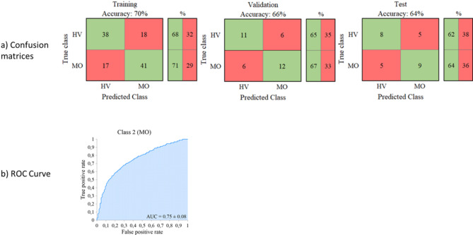
Results: Both models demonstrated robust performance, achieving over 68% in all the performance metrics (accuracy, sensitivity, specificity, and F1 scores). The classification model trained with FFS-derived features performed better than the model trained with PCA results in distinguishing patients with MO from HV. The model trained with FFS-derived features achieved a median accuracy of 72.8% and an area under the curve (AUC) of 0.79, while the model trained with PCA results showed a median accuracy of 68.9% and an AUC of 0.75.

Conclusion: Our findings suggest that ANNs trained with SSEP-derived variables hold promise as a noninvasive tool for migraine classification, offering potential for clinical application and deeper insights into migraine diagnostics.

Keywords: Artificial intelligence; Evoked potentials; Habituation; Neurophysiology; Sensitization; Thalamus.

Fig. 1

Pipeline of the Artificial Neural Network (AANs) development. Somatosensory evoked potentials (SSEPs) were recorded by stimulating the median nerve at the wrist in both healthy volunteers (HV) and interictal episodic migraine patients (MO). The recordings were analyzed offline to extract low-frequency responses (LF-SSEPs) and high-frequency oscillations (HFO) from the cortical components of the somatosensory evoked potentials. Eleven features were extracted from the analysis, and two techniques were independently applied to reduce the dimensionality and select the relevant features: Principal Component Analysis (PCA) and Forward Feature Selection (FFS). PCA selected four relevant linear combinations of the features, while FFS selected three relevant features. Two different neural network models were trained with these features transferred to the input layer. The hidden layer comprised 50 neurons, while the output layer comprised 2 neurons. Both models were trained one hundred times by randomly dividing our dataset into training, validation, and test sets for each run. Finally, the performance of both models in classifying HV from MO was evaluated by calculating the median accuracy, the sensitivity (recall), the specificity, and the F1 score. The outcomes were derived by averaging the outputs from 100 neural networks trained on the same dataset. Created in BioRender. Sebastianelli, G. (2025) https://BioRender.com/l67q659

Fig. 2

a) Explained variance (%) by each component. The sum of the variance of the first four components accounts for almost 95% of the total variance. b) Number of principal components vs. accuracy. The value of the accuracy is based on the test dataset in order to evaluate the network’s robustness in terms of generalization capability

Fig. 3

a) Confusion matrices for a detailed summary of the ANN’s performance trained with the transformed features from Principal Component Analysis (PCA). The matrix is structured such that the rows represent the true classes (HV or MO), and the columns represent the predicted classes. The diagonal elements (in green) reflect the number of correctly classified cases (true negatives and true positives: TN - TP), while the off-diagonal elements (in red) capture the number of misclassifications (false negatives and false positives: FN - FP). A row summary displays the percentages of correctly and incorrectly classified observations for each true class. For example, considering the training dataset, in the row corresponding to the “HV” class, the percentage of HV correctly classified is shown along with the percentage of HV misclassified as having MO (TN = 68%; FP = 32%). Similarly, for the “MO” class, the row summary indicates the percentage of individuals correctly identified as having MO (TP = 71%) and those misclassified as HV (FN = 29%). b) Area under the curve (AUC) for the overall performance of the ANN trained with the transformed features from PCA. The ROC curve is a graphical representation that illustrates the performance of a binary classifier across different threshold settings. The ROC curve plots the True Positive Rate (TPR) on the y-axis against the False Positive Rate (FPR) on the x-axis for all possible threshold values. As the threshold varies, the trade-off between correctly classifying positive cases and misclassifying negative cases as positive is visualized. An ideal classifier would achieve a point near the top-left corner of the ROC plot, where the TPR is high, and the FPR is low. Furthermore, the AUC provides a single metric that summarizes the classifier’s overall performance. An AUC of 1 represents perfect classification, where the classifier achieves a high TPR with a low FPR across all thresholds. An AUC of 0.5, however, indicates performance no better than random chance

Fig. 4

Feature selection frequency of the 11 considered variables obtained by training 100 neural networks. The green columns indicate the selected features for training the ANN

Fig. 5

a) Confusion matrices for a detailed summary of the ANN’s performance trained with the Forward Feature Selection (FFS). The matrix is structured such that the rows represent the true classes (HV or MO), and the columns represent the predicted classes. The diagonal elements (in green) reflect the number of correctly classified cases (true negatives and true positives: TN and TP), while the off-diagonal elements (in red) capture the number of misclassifications false negatives and false positives: FN - FP). A row summary displays the percentages of correctly and incorrectly classified observations for each true class. For instance, considering the training dataset, in the “HV” class row, the percentage of correctly classified HV is displayed alongside the percentage misclassified as having MO (TN = 75%; FP = 25%). Similarly, for the “MO” class, the row summary reflects the percentage of individuals correctly identified as having MO (TP = 72%), and those misclassified as HV (FN = 28%). b) Area under the curve (AUC) for the overall performance of the ANN trained with the features selected with the FFS

References

1. Steiner TJ, Stovner LJ (2023) Global epidemiology of migraine and its implications for public health and health policy. Nat Rev Neurol 19:109–117. 10.1038/s41582-022-00763-1 - PubMed
1. Steiner TJ, Stovner LJ, Jensen R et al (2020) Migraine remains second among the world’s causes of disability, and first among young women: findings from GBD2019. J Headache Pain 21:137. 10.1186/s10194-020-01208-0 - PMC - PubMed
1. Ashina M, Terwindt GM, Al-Karagholi MA-M et al (2021) Migraine: disease characterisation, biomarkers, and precision medicine. Lancet 397:1496–1504. 10.1016/S0140-6736(20)32162-0 - PubMed
1. (2018) Headache Classification Committee of the International Headache Society (IHS) The International Classification of Headache Disorders, 3rd edition. Cephalalgia 38:1–211. 10.1177/0333102417738202 - PubMed
1. Puledda F, Viganò A, Sebastianelli G et al (2023) Electrophysiological findings in migraine May reflect abnormal synaptic plasticity mechanisms: A narrative review. Cephalalgia 43:3331024231195780. 10.1177/03331024231195780 - PubMed
LinkOut - more resources