Test allocation based on risk of infection from first and second order contact tracing

Abstract

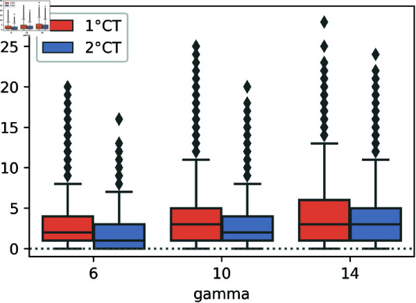
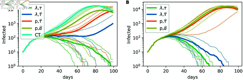
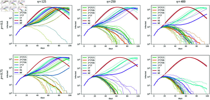
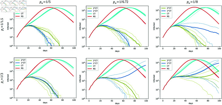
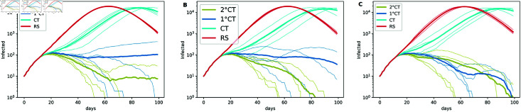
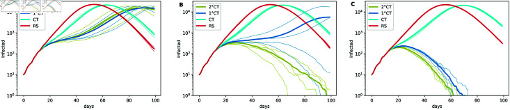
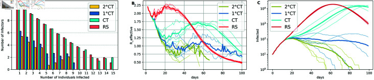
Strategies such as testing, contact tracing, and quarantine have been proven to be essential mechanisms to mitigate the propagation of infectious diseases. However, when an epidemic spreads rapidly and/or the resources to contain it are limited (e.g., not enough tests available on a daily basis), to test and quarantine all the contacts of detected individuals is impracticable. In this direction, we propose a method to compute the individual risk of infection over time, based on the partial observation of the epidemic spreading through the population contact network. We define the risk of individuals as their probability of getting infected from any of the possible chains of transmission up to length-two, originating from recently detected individuals. Ranking individuals according to their risk of infection can serve as a decision-making tool to prioritise testing, quarantine, or other preventive measures. We evaluate interventions based on our risk ranking through simulations using a fairly realistic agent-based model calibrated for COVID-19 epidemic outbreak. We consider different scenarios to study the role of key quantities such as the number of daily available tests, the contact tracing time-window, the transmission probability per contact (constant versus depending on multiple factors), and the age since infection (for varying infectiousness). We find that, when there is a limited number of daily tests available, our method is capable of mitigating the propagation more efficiently than some other approaches in the recent literature on the subject. A crucial aspect of our method is that we provide an explicit formula for the risk, avoiding the large number of iterations required to achieve convergence for the algorithms proposed in the literature. Furthermore, neither the entire contact network nor a centralised setup is required. These characteristics are essential for the practical implementation using contact tracing applications.

Fig 1. Interactions between individuals over three days.

When the individual A is detected, A is quarantined, and their time of infection is estimated. The $2^{\circ }$contact tracing method traces forward the first and second contacts in interaction with A after the estimated time of infection. The risk for these individuals is then computed, and those with the highest risk are selected for testing.

Fig 2. Effect of the estimators τ^Ii (blue), α^Ii (orange), and the real time of infection τIi (green).

(A) The $1^{\circ }$CT method with parameter γ = 6. (B) $2^{\circ }$CT with γ = 6 and ζ = 7. (C) $2^{\circ }$CT with γ = 6 and ζ = 8. (D) $2^{\circ }$CT with γ = 6 and ζ = 9. The figures illustrate the impact of these methods on the spread of the epidemic, displaying the number of infectious individuals over T = 100 days in a population of size N = 50K. The intervention begins on day $t_0=12$, with $N_0=10$ initial patients (patient zero cases), η = 125 daily available tests, a proportion $p_s=1$ of detected severe symptomatic individuals, and a proportion $p_m=0.75$ of detected mild symptomatic individuals.

Fig 3. Comparison of infection time estimators.

Box plots of the differences ${\tau }_I^i-{\hat{\tau }}_I^i$ (orange) and ${\tau }_I^i-{\hat{\alpha }}_I^i$ (blue) for individuals detected by risk using the $1^{\circ }$CT and $2^{\circ }$CT methods, considering the parameter range ζ = 7 , 8 , 9 and γ = 6. Each box plot was generated using four seeds, with parameters T = 100, N = 50K, $t_0=12$, $N_0=10$, η = 125, $p_S=1$, and $p_m=0.75$.

Fig 4. Effect of γ on epidemic spread.

Effect of γ on epidemic spread for strategies $1^{\circ }$CT (blue) and $2^{\circ }$CT (yellow) when ζ = γ + 3, with (A) γ = 6, (B) γ = 10, and (C) γ = 14. Each plot was generated using four seeds, with parameters T = 100, N = 50K, $t_0=12$, $N_0=10$, η = 125, $p_S=1$, and $p_m=0.75$.

Fig 5. Box plots of infection and detection time differences.

Box plots of the differences between the time of infection and the time of detection for individuals detected by risk using the $1^{\circ }$CT and $2^{\circ }$CT methods, with parameter values γ = 6 , 10 , 14, and for $2^{\circ }$CT with ζ = γ + 3. The simulations were performed with T = 100, N = 50K, $t_0=12$, $N_0=10$, η = 125, $p_S=1$, and $p_m=0.75$, using four different seeds.

Fig 6. Effect of the transmission probability function on epidemic spread.

Effect of the transmission probability function on the spreading of the epidemic for the (A) $1^{\circ }$CT and (B) $2^{\circ }$CT methods. Each plot was generated with T = 100, N = 50K, $t_0=12$, $N_0=10$, η = 125, $p_m=0.75$, $p_S=1$, γ = 6, and for $2^{\circ }$CT with ζ = 9.

Fig 7. Effect of η and pm on epidemic spread.

Effect of the parameters η (the number of daily available tests, increasing from left to right) and $p_m$ (the proportion of daily detected individuals with mild symptoms, increasing from top to bottom) on epidemic spread for the strategies $1^{\circ }$CT, $2^{\circ }$CT, CT, RS, and MF. In all simulations, we consider T = 100, N = 50K, $t_0=12$, $N_0=10$, and $p_S=1$. The estimation of the infection time for the $1^{\circ }$CT and $2^{\circ }$CT strategies is given by ${\hat{\tau }}_I^i$. We fix the parameters γ = 6 and ζ = 7 , 8 , 9 (indicated in the legend as $2^{\circ }$CT(7), $2^{\circ }$CT(8), and $2^{\circ }$CT(9), respectively). The parameter values for the MF strategy are ${\rho }_{MF}=5$ and $t_{MF}=10$.

Fig 8. Effect of pm and ps on epidemic spread.

Effect of the parameters $p_m$ (the daily detection probability of individuals with mild symptoms, decreasing from left to right) and $p_s$ (the daily detection probability of individuals with severe symptoms, decreasing from top to bottom) on epidemic spread for the strategies $1^{\circ }$CT, $2^{\circ }$CT, CT, and RS. Each plot is generated from simulations using four seeds, with parameters T = 100, N = 50K, $t_0=12$, $N_0=10$, and η = 400. The estimation of the infection time for the $1^{\circ }$CT and $2^{\circ }$CT strategies is given by ${\hat{\tau }}_I^i$. We fix the parameters γ = 6 and ζ = 9.

Fig 9. Effect of sensitivity and specificity on epidemic spread.

Effect of sensitivity and specificity on epidemic spread for the strategies $1^{\circ }$CT, $2^{\circ }$CT, CT, and RS with (A) η = 450, (B) η = 500, and (C) η = 600. Each plot was generated from simulations using four seeds, with parameters T = 100, N = 50K, $t_0=12$, $N_0=10$, $p_s=1$, and $p_m=1∕3$. The estimation of the infection time for the $1^{\circ }$CT and $2^{\circ }$CT strategies is given by ${\hat{\tau }}_I^i$. We fix the parameters γ = 6 and ζ = 9.

Fig 10. Effect of the quarantine adoption fraction q on epidemic spread.

Effect of the parameter q (the fraction of individuals adopting quarantine), increasing from left to right with (A) q = 0 . 9, (B) q = 0 . 95, and (C) q = 1, on epidemic spread for the strategies $1^{\circ }$CT, $2^{\circ }$CT, CT, and RS. Each plot was generated from simulations using four seeds, with parameters T = 100, N = 50K, $t_0=12$, $N_0=10$, η = 450, $p_m=1∕5$, and $p_s=1∕3$. The estimation of the infection time for the $1^{\circ }$CT and $2^{\circ }$CT strategies is given by ${\hat{\tau }}_I^i$. We fix the parameters γ = 6 and ζ = 9.

Fig 11. Effect of super-spreaders on ranking methods.

Effect of super-spreaders on the ranking methods $1^{\circ }$CT, $2^{\circ }$CT, CT, and RS based on (A) the frequency of secondary infections caused by index cases, (B) the effective reproduction number over time ($R_{\text{effective}}$), and (C) the number of infectious individuals over time. Each plot was generated from simulations using four seeds, with parameters T = 100, N = 50K, $t_0=12$, $N_0=10$, η = 500, $p_m=1∕3$, $p_s=1$, q = 1, sensitivity = 0.9, and specificity = 0.95. The estimation of the infection time for the $1^{\circ }$CT and $2^{\circ }$CT strategies is given by ${\hat{\tau }}_I^i$. Parameters γ = 6 and ζ = 9 are fixed across all simulations.

References

1. Brandt AM. The history of contact tracing and the future of public health. Am J Public Health 2022;112(8):1097–9. doi: 10.2105/ajph.2022.306949 - DOI - PMC - PubMed
1. Baker A, Biazzo I, Braunstein A, Catania G, Dall’Asta L, Ingrosso A, et al.. Epidemic mitigation by statistical inference from contact tracing data. Proc Natl Acad Sci USA 2021;118(32):e2106548118. doi: 10.1073/pnas.2106548118. - DOI - PMC - PubMed
1. Herbrich R, Rastogi R, Vollgraf R. CRISP: a probabilistic model for individual-level COVID-19 infection risk estimation based on contact data. arXiv. 2022. https://arxiv.org/abs/2006.04942
1. Batlle P, Bruna J, Fernandez-Granda C, Preciado VM. Adaptive test allocation for outbreak detection and tracking in social contact networks. SIAM J Control Optim. 2022;60(2):S274–93. doi: 10.1137/20m1377874 - DOI
1. Romijnders R, Asano YM, Louizos C, Welling M. No time to waste: practical statistical contact tracing with few low-bit messages. In Proceedings of The 26th International Conference on Artificial Intelligence and Statistics, PMLR; 2023. pp. 7943–60. Available: https://proceedings.mlr.press/v206/romijnders23a.html.