A beginner's approach to deep learning applied to VS and MD techniques

Abstract

It has become impossible to imagine the fields of biochemistry and medicinal chemistry without computational chemistry and molecular modelling techniques. In many steps of the drug development process in silico methods have become indispensable. Virtual screening (VS) can tremendously expedite the early discovery phase, whilst the use of molecular dynamics (MD) simulations forms a powerful additional tool to in vitro methods throughout the entire drug discovery process. In the field of biochemistry, MD has also become a compelling method for studying biophysical systems (e.g., protein folding) complementary to experimental techniques. However, both VS and MD come with their own limitations and methodological difficulties, from hardware limitations to restrictions in algorithmic capabilities. One solution to overcoming these difficulties lies in the field of machine learning (ML), and more specifically deep learning (DL). There are many ways in which DL can be applied to these molecular modelling techniques to achieve more accurate results in a more efficient manner or expedite the data analysis of the acquired results. Despite steadily increasing interest in DL amidst computational chemists, knowledge is still limited and scattered over different resources. This review is aimed at computational chemists with knowledge of molecular modelling, who wish to possibly integrate DL approaches in their research and already have a basic understanding of the fundamentals of DL. This review focusses on a survey of recent applications of DL in molecular modelling techniques. The different sections are logically subdivided, based on where DL is integrated in the research: (1) for the improvement of VS workflows, (2) for the improvement of certain workflows in MD simulations, (3) for aiding in the calculations of interatomic forces, or (4) for data analysis of MD trajectories. It will become clear that DL has the capacity to completely transform the way molecular modelling is carried out.

Fig. 1

Overview of the DEEPScreen architecture. Each prediction model included in DEEPScreen takes as input small molecule ligands in the form of SMILES representations, transforms them into 200-by-200 pixel 2D structural images, and then runs a predictive CNN model on them in order to predict whether these ligands are either active (i.e., interacting) or inactive (i.e., non-interacting) against a specific target protein [36]

Fig. 2

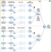
Overview of the DeepScreening workflow employed by Joshi et al. for the screening of natural compounds against 3CL^pro. Through a LBVS step employing a DL predictive model, a SBVS step employing a traditional molecular docking method, additional in silico screenings for characteristics such as pharmacokinetics and toxicity, and MD simulations, a database of 1,611 compounds was narrowed down to two specific hit compounds for further testing [39]

Fig. 3

Overview of the GAN architecture developed by Andrianov et al. for the in silico generation of HIV-1 entry inhibitors. The generator consists of an AE model capable of analyzing molecular fingerprint input and generating new synthetic fingerprints through sampling of its learned latent space. This learned latent space is further optimized through adversarial learning with the discriminator, which gets taught to distinguish the latent space from random normal distribution data. After training and optimization, the generator was used to obtain synthetic fingerprints of strong binders against the HIV-1 viral envelope protein gp120, which were sought out in a chemical library through a fingerprint similarity search for further testing [47]

Fig. 4

Overview of the workflow employed by Arshia et al. for the in silico compound generation of 3CL^pro inhibitors. An LSTM RNN architecture was trained through DTL for the generation of 3CL^pro binding molecules. Each generation step, the generated molecules were further validated and tested using traditional molecular docking methods. A genetic algorithm then selected a limited number of compounds for further finetuning of the RNN model. After ten generation steps, all molecules with high binding affinity for 3CL^pro were clustered through a hierarchical clustering method, and the compounds with the highest binding affinity in each cluster were selected for further testing [53]

Fig. 5

Overview of the DeepBindRG architecture and the external validation carried out on this DL model by Zhang et al. [81] Crystallized protein–ligand complexes from the PDBbind 2018 database were used as training, validation, and internal test sets for DeepBindRG: a CNN model based on the ResNet architecture. Datapoints were fed to the network as 2D binding interface-related matrices and eventually led to an output prediction of the binding affinity of the ligand to the protein. After training and internal validation, DeepBindRG was further validated using external datasets with either known or unknown native protein–ligand conformations. When unknown, the traditional molecular docking method AutoDock Vina was used to generate the binding complex

Fig. 6

Overview of the DiffDock architecture by Corso et al. [110] When given separate ligand and protein structures as input, the DL model employs a reverse diffusion process to step-by-step sample more realistic binding poses and refine the system towards binding poses as optimal as possible. A confidence model is then employed on each final binding pose to predict their confidence and provide the top ranked poses

Fig. 7

Overview of the generative AE architecture developed by Degiacomi [137]. Of a protein of interest, the flattened Cartesian coordinates of a dataset of conformations are fed to the AE model as input. After learning, the latent space is a low-dimensional representation of the conformational space of the protein. Through interpolation, it now becomes possible to generate new protein conformations, which can be used as starting conformations for other in silico techniques, such as molecular docking or MD simulations

Fig. 8

Overview of the MD/DL iterative workflow developed by Ma et al. for protein folding problems, employing a CVAE architecture [139]. MD simulations are run in parallel for a protein of interest. The conformations generated throughout these simulations are fed to the CVAE as flattened Cartesian coordinates. After learning, the latent space is a low-dimensional representation of the conformational space of the protein, with regions defined by specific latent features/characteristics. This can be used to sample conformations with certain latent features (e.g., the RMSD of a conformation compared to the folded native state/unfolded starting state). Based on these samples, specific simulation runs can be terminated, and new runs can be started from the sampled conformations, in order to speed up the protein folding process

Fig. 9

Overview of 1st generation NNP architectures, which consist of DFCNNs taking as input the Cartesian coordinate vector of the N atoms of a system of interest and output a potential energy prediction for that system [153]

Fig. 10

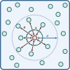
Schematic representation of radial and angular ACSFs [153]. In this example, the ACSFs are defined for the central atom (red circle) of the system (blue box). A cut-off radius C (blue dotted line) defines which neighboring atoms (green circles) are included in the atomic environment of the central atom, and thus in the calculation of the ACSFs. The radial ACSF is the sum of the products of Gaussians and cut-off functions for all atoms within the atomic environment, with the Gaussians describing the distances R between the central atom and each neighboring atom (red arrows), whilst the cut-off functions ensure decay to zero in value and slope towards the cut-off radius. The angular ACSF is the sum of the products of the cut-off functions and the angles A between the central atom and pairs of two neighboring atoms (green curved arrows)

Fig. 11

A Overview of 2nd generation HDNNP architectures, in which the Cartesian coordinate vectors of the atoms of a system of interest get converted into a vector of ACSFs, to form the input for individual atomic NNs. These DFCNNs predict the potential energy of each separate atom in the system, delivering the total potential energy of the system when these atomic energies get tallied up. The atomic NNs are trained in the same manner per chemical element. B Overview of 3rd generation HDNNP architectures, expanding upon 2nd generation HDNNPs by not only using atomic NNs to predict atomic potential energies per atom of a system, but also atomic charge NNs to predict atomic electrostatic energies. This enables the NNPs to describe more long-range interactions in the system. The short-range potential energies and total electrostatic energies are summed up to provide the total energy of the system. The atomic charge NNs are trained in a different manner per chemical element than atomic NNs [153]

Fig. 12

Overview of 4th generation HDNNP architectures, similar to 3rd generation HDNNPs in the prediction of both atomic charges and atomic potential energies using separate atomic NNs. In this generation, the atomic charge NNs first predict atomic electronegativities that are converted to atomic charges through a charge equilibration scheme depending on the global system of interest. The atomic charges then form an extra level of input for the atomic NNs predicting the short-range atomic potential energies. These two added elements ensure that the architecture considers non-local charge dependencies, resulting in a more accurate total potential energy prediction [153]

Fig. 13

Overview of the concept of “active learning” [153]. NNP models with differentiating parameters are trained on an initial reference dataset, attempting to capture all the atomic environments relevant for the system of interest to be simulated. Through validation of these models, it is possible to determine what data needs to be added to the reference datasets for further refinement of the NNP models. The models try to learn to describe an unknown potential energy landscape (red and green curves vs. black curve of top right graph). In the conformational regions where the predicted curves differentiate, more information should be provided to the models. These conformations can be obtained through additional MD simulations of the reference structures to provide additional atomic environments for further training. When all trained models converge to describe one potential energy curve (overlapping curves of bottom right graph), the NNPs are optimized, and a final architecture can be selected for the actual application

Fig. 14

Overview of the MD trajectory data analysis workflow developed by Plante et al. [174] Ligands representing functionally-selective classes (e.g., full agonists, inverse agonists, partial agonists) are docked onto proteins of interest to create systems for MD simulations. Relevant frames from those simulations are selected for the development of DL training datasets. From these frames the ligand atoms are extracted, but a label is provided with each frame detailing the class of the ligand previously bound in the conformation to allow loss optimization. The protein conformations undergo a positional and orientational structure scrambling procedure to remove bias, after which they are translated into a 2D picture-like format. Each pixel in a picture represents an atom of the protein conformation, with its RGB values corresponding to the XYZ coordinates of the atom. A CNN model based on the DenseNet architecture is then developed and trained on the pictures and class labels to predict the label of the ligand that was bound in a conformation. After optimization, the network’s decisions can be analyzed using saliency mapping, as to show the protein regions/structural features relevant for the binding of different ligands

Fig. 15

Overview of the DL-RP-MDS method developed by Tam et al. [183]. To measure the impact of missense variations on protein function, an AE architecture was built and trained. It takes as input the Ramachandran plots of conformations of the query protein with a missense variation of interest, generated using MD simulations. Through its reconstruction of the input via its encoder and decoder layers, it learns a low-dimensional latent representation of the Ramachandran plot input data. This latent space forms the input of a DFCNN classifier that predicts the variants of the protein to either be deleterious or undefined (i.e., benign)

References

1. Wang J, Bhattarai A, Do HN, Miao Y (2022) Challenges and frontiers of computational modelling of biomolecular recognition. QRB Discov 3:1–12. 10.1017/QRD.2022.11 - PMC - PubMed
1. Hollingsworth SA, Dror RO (2018) Molecular dynamics simulation for All. Neuron 99:1129–1143. 10.1016/J.NEURON.2018.08.011 - PMC - PubMed
1. De Vivo M, Masetti M, Bottegoni G, Cavalli A (2016) Role of molecular dynamics and related methods in drug discovery. J Med Chem 59:4035–4061. 10.1021/ACS.JMEDCHEM.5B01684 - PubMed
1. Amini A, Amini A, Lolla S. (2024) MIT 6.S191 | Introduction to deep learning. http://introtodeeplearning.com/.
1. Abadi M, Agarwal A, Barham P, Brevdo E, Chen Z, Citro C et al (2016) TensorFlow: large-scale machine learning on heterogeneous distributed systems. ArXiv. 10.48550/arXiv.1603.04467
LinkOut - more resources