CAVE: Connectome Annotation Versioning Engine

Abstract

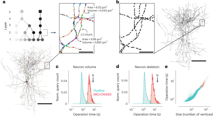
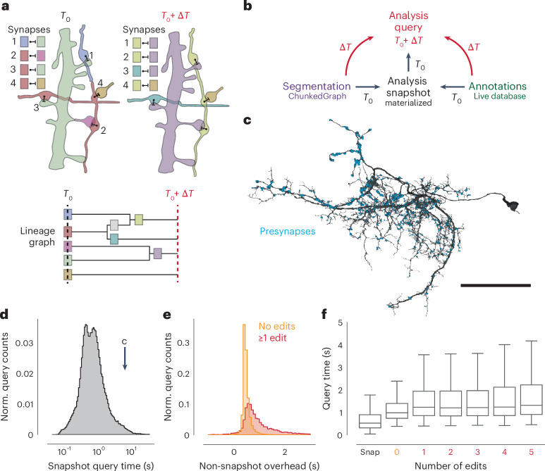
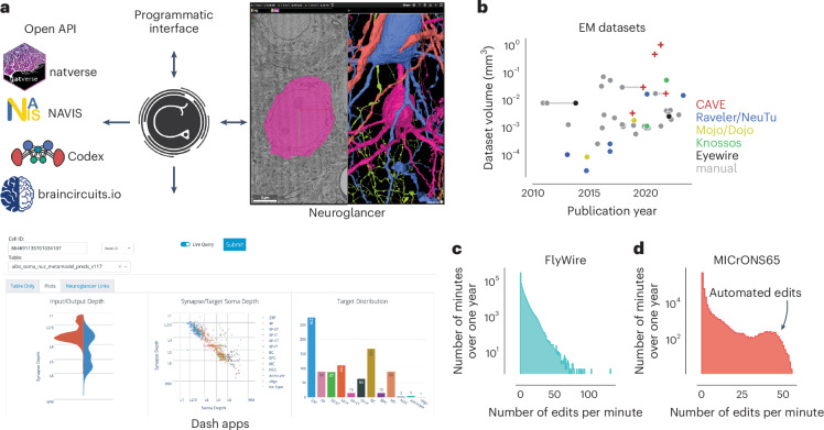
Advances in electron microscopy, image segmentation and computational infrastructure have given rise to large-scale and richly annotated connectomic datasets, which are increasingly shared across communities. To enable collaboration, users need to be able to concurrently create annotations and correct errors in the automated segmentation by proofreading. In large datasets, every proofreading edit relabels cell identities of millions of voxels and thousands of annotations like synapses. For analysis, users require immediate and reproducible access to this changing and expanding data landscape. Here we present the Connectome Annotation Versioning Engine (CAVE), a computational infrastructure that provides scalable solutions for proofreading and flexible annotation support for fast analysis queries at arbitrary time points. Deployed as a suite of web services, CAVE empowers distributed communities to perform reproducible connectome analysis in up to petascale datasets (~1 mm³) while proofreading and annotating is ongoing.

Fig. 1. Proofreading and analysis of connectomics datasets.

a, A rich set of ultrastructural features can be extracted from EM images and used for analysis. The corresponding ultrastructural features are annotated with a red asterisk (*). The synapse is annotated with a red arrow pointing from the presynaptic site to the postsynaptic site. b, Large connectomics datasets are proofread, annotated and analyzed by a distributed pool of users in parallel. c, Proofreading adds and removes fragments from cell segments (left, before proofreading; center, removed and added fragments; right, after proofreading). d, Synapse assignments have to be updated with proofreading. All synapses (within the cutout) that were added and removed though the proofreading process of the cell in c are shown. Scale bars, 100 µm (c), 1 µm (a: synapse, mitochondria), 10 µm (a: nuclei) and 20 µm (d). T, time.

Fig. 2. Scaling the ChunkedGraph to petascale datasets.

a, Automated segmentation overlaid on EM data. Each color represents an individual putative cell. b, Different colors represent supervoxels that make up putative cells. c, Supervoxels belonging to a particular neuron, with an overlaid cartoon of its supervoxel graph. These data corresponds to the framed square in a and the full panel in b. d, One-dimensional representation of the supervoxel graph. The ChunkedGraph data structure adds an octree structure to the graph to store the connected component information. Each abstract node (black nodes in levels >1) represents the connected component in the spatially underlying graph. e, Storage and costs for the supervoxel graph storage under the original and the improved implementation (v2); GCS, Google cloud storage; TB, terabytes. f, To submit a split operation, users place labels for each side of the split (top right). The backend system first connects each set of labels on each side by identifying supervoxels between them in the graph (left). The extended sets are used to identify the edges needed to be cut with a maximum-flow minimum-cut algorithm. g, Examples of graph traversals for looking up the root ID for a supervoxel ID (top) and supervoxel IDs for a root ID within a spatially defined search area (bottom). Note that only part of the graph needs to be traversed. h,i, Performance measurement from real-world user interactions measured on the ChunkedGraph server for different types of reads (h) and edits (i). The cumulative ratio of all measured interactions for a given response time is plotted on the y axis. Scale bar, 500 nm.

Fig. 3. Fast calculation of morphological features and skeletons.

a, The basket cell from Fig. 1c broken into L2 chunks where each chunk is colored differently. For each chunk, the L2-Cache stores a number of features, such as area, volume and representative coordinate. b, A skeleton derived from the ChunkedGraph and L2-Cache without consulting the segmentation data. c, Client-side timings for calculating neuron volumes using ChunkedGraph and L2-Cache for neurons in FlyWire and MICrONS65 (N_FlyWire = 101,554; N_MICrONS65 = 1,357). The timing for the neuron in b is highlighted. d, Client-side timings for creating skeletons from ChunkedGraph and L2-Cache (N_FlyWire = 78,030; N_MICrONS65 = 1,357). Norm., normalized. e, Client-side timings for creating skeletons plotted against the size of the skeletons. Each dot is a query for a single neuron (see d for the number of samples). Scale bars, 100 µm (insets: scale bar, 5 µm).

Fig. 4. Annotations for proofreadable datasets.

a, Spatial points can be used to capture a huge diversity of biological metadata generated by either human annotators or machine algorithms. Additional metadata for existing CAVE annotations can be added with reference annotations that avoid duplicating existing annotations (illustrated as dashed lines). b, The annotation services handle all annotations through a generic workflow that depends only on expressing all annotations as collections of spatial points and associated metadata. Spatial annotations mark the location of a feature, such as a spine head. Scale bar, 500 nm. c, The materialization service retrieves the supervoxel ID underlying all spatial points. d, This enables the materialization service to look up the root ID underneath that points at any given moment in time using the ChunkedGraph. e, Illustration of how the mapping from supervoxel ID to segment ID changed the annotation due to proofreading (octree levels not shown). The changes are tracked in a lineage graph of the altered roots.

Fig. 5. Querying the dataset for any time point.

a, Edits change the assignment of synapses to segment IDs. Each of the four synapses is assigned to the segment IDs (colors) according to the presynaptic and postsynaptic points (point, bar). The identity of the segments changes through proofreading (time passed: ΔT) indicated by different colors. The lineage graph shows the current segment ID (color) for each point in time. b, Analysis queries are not necessarily aligned to exported snapshots. Queries for other time points are supported by on-the-fly delta updates from both the annotations and segmentation through the use of the lineage graph. c, A neuron in FlyWire with all its automatically detected presynapses. d, Time measurements for snapshot aligned queries of presynapses for proofread neurons in FlyWire (N = 121,400). e, Difference between the snapshot and nonsnapshot aligned presynapse queries. The two distributions differentiate cases without any edits to the queried neurons and cases with at least one edit to the queried neuron (N_{no edits} = 98,367; N_{≥1 edit} = 8,132). f, Presynapse query times for snapshot and nonsnapshot aligned queries, including cases where neurons were proofread with multiple edits. The horizontal bar is the median. Boxes are interquartile ranges, and whiskers are set at 1.5× the interquartile range. Number of samples by number of edits: snap, n = 121,389; 0, n = 137,866; 1, n = 7,074; 2, n = 3,512; 3, n = 2,074; 4, n = 1,325; 5, n = 850. Scale bar, 50 µm.

Fig. 6. Integration into connectomics projects.

a, CAVE supports multiple interfaces. In addition to programmatic access, users can explore and edit the data in CAVE interactively through neuroglancer or CAVE’s dash apps. CAVE integrates with existing and new tools for connectomics through packages such as natverse, Codex and braincircuit.io. b, Datasets published since 2010 by volume and year (volume is plotted on a log scale). Datasets that were published with manual and semiautomated means are connected with a horizontal gray line (Supplementary Table 2). c,d, Proofreading rate in edits per minute for FlyWire (N = 1,349,955; c) and MICrONS65 over 1 year of proofreading (N = 457,285; d).

Extended Data Fig. 1. Translating user inputs to graph splits.

(a) Bipartite split labels are applied to locations in space. (b) The closest supervoxels to label points are identified (red/blue dots). The supervoxel graph in the neighborhood of the labeled points is computed (graph), weighted by affinity between supervoxels. (c) Vertices along the shortest paths between each pair of red/blue labels are found (black dots and edges). Backup methods prevent overlap between paths. (d) Affinity between vertices along shortest paths is set to infinity and min cut is computed on the path-augmented supervoxel graph.

Extended Data Fig. 2. ChunkedGraph performance measurements on FlyWire.

These measurements are from the improved ChunkedGraph implementation using the same FlyWire supervoxel graph that was used for the original implementation. (a) Performance measurement from real-world user interactions measured on the ChunkedGraph server for reads, specifically leaves to root (median=41 ms, N = 13,410) and root leaves (median=55 ms, N = 50,001) operations, and (b) edits, specifically merge (median=2,734 ms, N = 4,189) and split (median=3,486 ms, N = 2,875) operations. The cumulative ratio of all measured interactions for a given response time is plotted in the y axis.

Extended Data Fig. 3. Overview of the core CAVE services, their storage and interactions.

Arrows indicate flow of data between services and storage backends. Services are implemented as microservices deployed through kubernetes.

Extended Data Fig. 4. Analysis of timings to calculate morphological features.

Each dot is a query for a single neuron. (a) Times to retrieve a list of L2 chunks for a neuron (root id). (b) Time to look up volume measurements for all L2 chunks belonging to a given neuron. (c) Total time to calculate volumes for neurons. Number of samples for all plots: N(FlyWire) = 101,554; N(MICrONS65) = 1,357.

Extended Data Fig. 5. Schematic of annotation databases, schemas, and annotation tables.

(a) Users can create and delete annotation tables through the annotation service. When creating a table, users select one of many available schemas that define the columns in the annotation table. (b) Users can create, update and delete annotations in the annotation table. The materialization service then adds these annotations to the associate segment table and regularly updates the root ids (that is, segment ids) associated with these annotations. (c) A commonly used schema for synapses. Each row defines a column in the annotation table. Entries of type BoundSpatialPoint are linked to the underlying segmentation and updated by the materialization service in the segment table. (d) Same as (c) but for a cell type schema. (e) Examples from an annotation table using the cell type schema from (d) in the MICrONS dataset.

Extended Data Fig. 6. Foreign key relationships between tables.

This example shows how annotation and segment tables for nucleus annotations are combined and further extended with reference tables. Annotation and segment tables are automatically combined by the Materialization service via a foreign key relationship on their ID columns. Reference tables created by the user also use foreign key relationships to associate additional information with rows in an annotation table. Multiple such reference tables can point at one Annotation table.

Extended Data Fig. 7. Annotation query timing analysis.

(a) Query times from Fig. 5d versus the size of the query in number of presynapses (N = 121,400). (b) Comparing snapshot and non-snapshot aligned presynapse queries for cases where the neuron was not edited between the snapshot and the query time (N = 121,367). The difference is the overhead of the mapping logic. The orange dashed line is a linear fit with intercept 0.44 s and a slope of 1.05.

Extended Data Fig. 8. Microservice organization into global and local clusters.

CAVE splits services into global and local clusters dependent on their function. Services in the global cluster are light-weight and usually support a wide array of datasets, provide general information about datasets, and user level authentication. Services on local clusters may require more resources and might be specific to a few datasets. Local clusters are usually limited to a list of datasets they can service and are associated with a global cluster. Multiple local clusters can be associated with the same global cluster.

References

1. Schubert, P. J. et al. SyConn2: dense synaptic connectivity inference for volume electron microscopy. Nat. Methods19, 1367–1370 (2022). - PMC - PubMed
1. Dorkenwald, S. et al. Automated synaptic connectivity inference for volume electron microscopy. Nat. Methods14, 435–442 (2017). - PubMed
1. Haberl, M. G. et al. CDeep3M-Plug-and-Play cloud-based deep learning for image segmentation. Nat. Methods15, 677–680 (2018). - PMC - PubMed
1. Wei, D. et al. MitoEM dataset: large-scale 3D mitochondria instance segmentation from EM images. Med. Image Comput. Comput. Assist. Interv.12265, 66–76 (2020). - PMC - PubMed
1. Heinrich, L. et al. Whole-cell organelle segmentation in volume electron microscopy. Nature599, 141–146 (2021). - PubMed
LinkOut - more resources