Functional connectomics spanning multiple areas of mouse visual cortex

Abstract

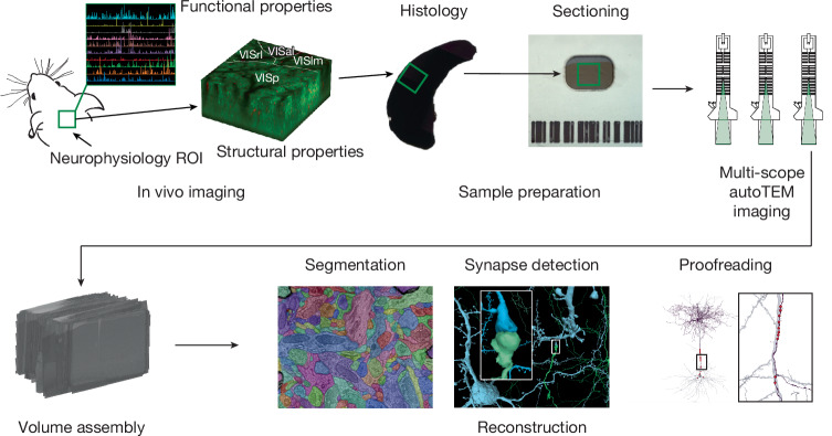
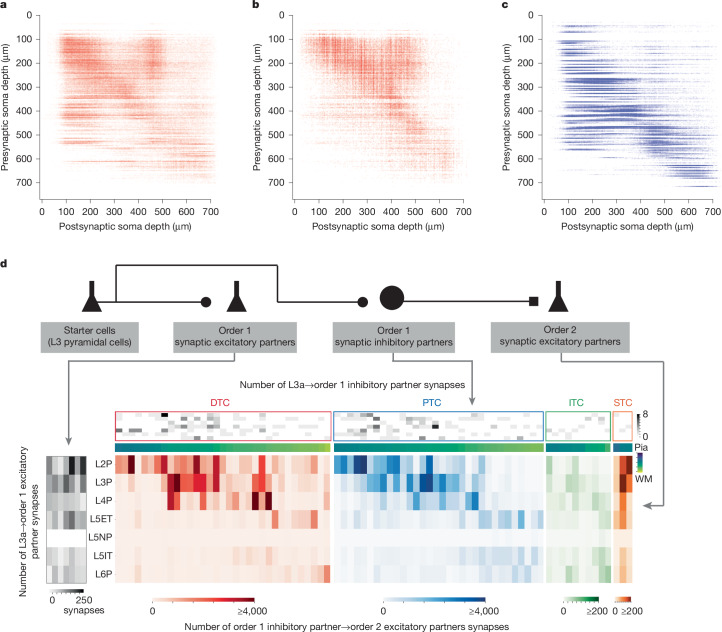
Understanding the brain requires understanding neurons' functional responses to the circuit architecture shaping them. Here we introduce the MICrONS functional connectomics dataset with dense calcium imaging of around 75,000 neurons in primary visual cortex (VISp) and higher visual areas (VISrl, VISal and VISlm) in an awake mouse that is viewing natural and synthetic stimuli. These data are co-registered with an electron microscopy reconstruction containing more than 200,000 cells and 0.5 billion synapses. Proofreading of a subset of neurons yielded reconstructions that include complete dendritic trees as well the local and inter-areal axonal projections that map up to thousands of cell-to-cell connections per neuron. Released as an open-access resource, this dataset includes the tools for data retrieval and analysis^1,2. Accompanying studies describe its use for comprehensive characterization of cell types^3-6, a synaptic level connectivity diagram of a cortical column⁴, and uncovering cell-type-specific inhibitory connectivity that can be linked to gene expression data^4,7. Functionally, we identify new computational principles of how information is integrated across visual space⁸, characterize novel types of neuronal invariances⁹ and bring structure and function together to uncover a general principle for connectivity between excitatory neurons within and across areas^10,11.

Fig. 1. Resource data type and data products.

a, The nine data resources that are publicly available at https://www.microns-explorer.org/. b, Relationship between different data types. The primary in vivo data resource consists of 2P calcium images, 2P structural images, natural and parametric video stimuli used as visual input, and behavioural measurements. The secondary (derived) in vivo data resource includes the responses of approximately 75,909 pyramidal cells from cortical layer 2 to 5 segmented from the calcium videos, along with the pupil position and diameter extracted from the video of eye movements and locomotion measured on a single-axis treadmill. The primary anatomical data are composed of ex vivo serial section transmission EM images registered with the in vivo 2P structural stack. The volume includes a portion of VISp and three higher visual areas—VISlm, VISrl and VISal—for all cortical layers except extremes of layer 1. The secondary anatomical data is derived from the serial section EM image stack, and consists of semi-automated segmentation of cells, automated segmentation of nuclei, and automatically detected synapses. The tertiary anatomical data consists of assignments of the synapses to presynaptic and postsynaptic cells, triangle meshes for these segments, classification of nuclei as neuronal versus non-neuronal, and classification of neurons into excitatory and inhibitory cell classes. Secondary data for co-registration of in vivo and ex vivo images consists of manually chosen correspondence points between 2P structural images and EM images. Tertiary co-registration data are a transformation derived from these correspondence points. The transformation is then used to facilitate the matching of cell indices between the 2P calcium cell segmentation masks and the EM segmentation cells. MicroCT, micro-computed tomography.

Fig. 2. Major experimental steps in the data acquisition workflow.

Outline of the major sequential steps used to generate the MICrONS dataset. First, in vivo measurements of neuronal functional properties are acquired from a region of interest (ROI) in the mouse visual cortex. In addition, a spatial overlapping in vivo structural image stack is collected to facilitate later registration with postmortem data. Following fixation of the brain, the tissue encompassing the functional ROI is processed for histology and sectioned. These sections are then imaged by TEM, and the resulting images are assembled into a 3D volume. Automated methods subsequently reconstruct the cellular processes and synapses within this volume, and the automated reconstructions are proofread as needed to ensure accuracy for further analysis. Image panels are adapted from Yin et al., Springer Nature Limited, and mouse and autoTEM drawings are adapted from Mahalingam et al., CC BY 4.0 (https://creativecommons.org/licenses/by/4.0/).

Fig. 3. In vivo calcium-imaging data.

a, Representation of the 2P functionally imaged volume with area boundaries (white) and vascular label from structural stack (red). b, Wireframe representation of 104 planes registered in the structural 2P stack. c, Mean depth of posterior (post.) and anterior (ant.) registered fields relative to the pial surface. d, 3D scatter plot of each functional mask in its registered location in the structural 2P stack. Black, VISp; red, VISlm; blue, VISal; green, VISrl. e, Example frames from each of the five stimulus types (cinematic, Sports-1M, rendered, Monet2 and Trippy) shown to the mouse. f, Raster of deconvolved calcium activity for three neurons to repeated stimulus trials (oracle trials; ten repeats of six sequential clips, with each repeat normalized independently). Rasters for high (top), medium (middle) and low (bottom) oracle scores with the percentile shown on the right. g, Trial-averaged raster (central 500 ms of trial-average raster for each direction, out of 937 ms) of deconvolved calcium activity for 80 neurons in 40 Monet2 trials (16 randomly ordered directions) grouped by preferred direction (5 neurons per direction; alternating blue shading) and sorted according to the stimulus directions.

Fig. 4. EM dataset.

a, Top view of EM dataset (grey) registered with the in vivo 2P structural dataset (vasculature in red and GCaMP in green). Area borders calculated from calcium imaging are shown as black lines. The two portions of the dataset are separated by a dashed line. Scale bar, 500 μm. Mouse drawing adapted from from Mahalingam et al., CC BY 4.0 (https://creativecommons.org/licenses/by/4.0/). b,c, Top view of small region showing the quality of the fine alignment and its robustness to large folds shown in c (the dataset is available at https://ngl.microns-explorer.org/#!gs://microns-static-links/mm3/data_fig/4b.json). Scale bars, 5 μm. d, Montage of a single section showing the coverage from pia to white matter and across three different cortical regions. Scale bar, 100 μm. e, Example of a single tile from the section shown in in d, with dashed squares representing the locations in f–h. Scale bar, 5 μm. f,g, Examples of excitatory synapses indicated with arrowheads (dataset available at https://ngl.microns-explorer.org/#!gs://microns-static-links/mm3/data_fig/4f.json (f) and https://ngl.microns-explorer.org/#!gs://microns-static-links/mm3/data_fig/4g.json (g)). h, Example of an inhibitory synapse (arrowhead) (dataset available at https://ngl.microns-explorer.org/#!gs://microns-static-links/mm3/data_fig/4h.json).

Fig. 5. Reconstruction.

a, A pyramidal cell reconstructed from the EM images (inset). b, Pyramidal cells from both subvolumes as they cross the subvolume boundary. c, A selection of 78 proofread pyramidal cells from subvolume 65. d, A distant pair of pyramidal cells connected by a synapse within subvolume 65.

Fig. 6. Integrated analysis resources and examples.

a–e, Cell body locations and cell-are type classifications, all nucleus detections shown in light grey. a, Non-neuronal cells, manually typed (dark outlines) and classifier-based (no outline). OPC, oligodendrocyte precursor cell. b, Excitatory cells, labelled by unsupervised clustering of morphological features (dark outline) and a model based on those labels. L2, layer 2; L3, layer 3; L4, layer 4; L5ET, layer 5 extratelencephalic; L5IT, layer 5 intratelencephalic; L5NP, layer 5 near-projecting; L6CT, layer 6 cortico-thalamic; L6IT, layer 6 intratelencephalic; L6WM, layer 6 white matter. c, Inhibitory cells, classified by human experts and trained models. d, Neurons registered to in vivo functional traces. e, Proofreading status of neurons in subvolume 65: black dots (fully proofread), red (cleaned of false merges but potentially incomplete) and blue (dendrites cleaned/extended). f, The number of output synapses per neuron shown in e versus the fraction mapped to a single postsynaptic soma, coloured by cell class. g, A fully proofread pyramidal cell (nucleus ID: 294657, segment ID: 864691135701676411) with postsynaptic soma locations shown as coloured dots (by cell class). Cells with functionally co-registered regions are outlined in dark green. h, Quantification of synapses associated with different categories of postsynaptic cells. The first column shows the fraction that map to a single postsynaptic soma. The second column shows the fraction of those that are excitatory or inhibitory. The third column shows the fraction of cells that are in each sub-class based on the model shown in b,c. The fourth column shows the proportion that map to functionally co-registered cells. The cell and its synapses are viewable at https://neuroglancer-demo.appspot.com/#!gs://microns-static-links/mm3/data_fig/6f.json. i, EM image (i) and corresponding image from the 2p structural stack (j) centred on the cell shown in g (yellow circle). Red arrowheads indicate blood vessels. k, Functional responses of the presynaptic (presyn) neuron (g; yellow) and its functionally co-registered postsynaptic (postsyn) targets. Heat maps show average ΔF/F traces for the presynaptic neuron and postsynaptic targets, sorted by synaptic strength, in response to oracle clips from functional scans.

Fig. 7. Connectivity matrices and analysis.

a–c, Connectivity matrix for proofread neurons connecting to all postsynaptic targets of the predicted class: excitatory→excitatory (a); excitatory→inhibitory (b); inhibitory→excitatory (c). Each connection between two cells is represented by a dot, with the position on the x axis depicting the depth of the postsynaptic soma and the position on the y axis depicting the depth of the presynaptic cell. Dots are transparent, with darker shades indicate more connections between laminar depths. Layer boundaries are shown as dashed grey lines. d, First-order and second-order synaptic output heat maps of seven layer 3 pyramidal cells similar to the one shown in Fig. 6g. Left, total number of synapses that each layer 3 pyramidal cell makes with each of their order 1 postsynaptic excitatory cell types. Greyscale heat map (top) showing number of synapses that each L3 pyramidal cell makes with their individual order 1 postsynaptic inhibitory partners, sorted by synaptic targeting types and soma depth from the pia to white matter (WM). Coloured heat map (bottom) showing total number of synapses that each order 1 inhibitory partner makes with each of their postsynaptic order 2 excitatory partners of layer 3 pyramidal cells, colour-coded by the synaptic targeting types of order 1 inhibitory partners. Inhibitory cell subclasses are represented as follows: DTC, distal targeting cells (also known as Martinotti cells); PTC, proximal targeting cells (also known as basket cells); ITC, inhibitory targeting cells; STC, sparse targeting cells (mostly neurogliaform). L3a, layer 3a.

Extended Data Fig. 1. Test Volume Locations for Validation of Automated Synapse Detection.

Location and distribution of test subvolumes (x = 5.5 µm, y = 5.5 µm, z = 5.5 µm) throughout the whole subvolume 65 that were used for validation of automated synaptic contact segmentation. Identification and annotation of synaptic contacts (n = 8,611 synapses) were performed manually within each subvolume and compared with automated results to calculate subvolume and combined precision (96%), recall (89%), and F1 scores (92%), with test subvolume F1 scores visualized by color within each plot. The two panels show a coronal (a) and top (b) view of the location of the sampling sites. In (a) the vertical axis represents the pia to white matter direction and the horizontal axis represents the medial-lateral direction. In (b) the vertical axis represents the anterior-posterior direction and the horizontal axis represents the medial-lateral direction.

Extended Data Fig. 2. Proofreading statistics across the volume.

(A) Histogram of number of edits across all the objects associated with nuclei. Distribution of neurons with complete dendritic proofreading highlighted in blue, and neurons with clean axons in orange. Cells with complete dendritic proofreading have often had some axon edits as well, so this is an upper bound on the number of edits required to fully extend dendrites. Most cells have had very little proofreading and have been mostly touched by automated methods. Note plot is on a log-log scale. (B) Number of edits compared to number of output synapses in reconstruction. For all the clean axons for which we have cell type annotations, the number of edits versus the number of outputs is plotted on a log log scale. Data points are colored with respect to their broad cell class. Generally, more extensively reconstructed axons have more edits, but there are also strong cell and cell-type specific effects. This reflects systematic differences in the thickness of axons of different cell types, as well as variation in how much of the axon is contained within the volume and the quality of the segmentation in different locations in the dataset.

Extended Data Fig. 3. Multi-Soma Proofreading.

(A) Distribution of multi-soma IDs by number of neuronal nuclei was monitored throughout proofreading. Difference in multi-neuron root IDs before APL proofreading (dark blue) and after (light blue). Note that this shows the number of neurons per ID, which means that non-neuron somas are not counted. This figure was derived using the soma classification table: nucleus_ref_neuron_svm. Note that a small number of multi-soma IDs were skipped during APL proofreading because they contain low quality neurons merged to myelinated axons or they were falsely classified as neuronal (e.g. blood vessels); (B) Spatial distribution of multi-neuron ID soma centers (soma locations of merged cells containing ≥ 2 neuronal nuclei) before APL proofreading and after. Both are a lateral view of the volume that shows distribution across layers, from pia (top) to white matter (bottom). Color-bar represents depth.

Extended Data Fig. 4. Manual co-registration metrics.

a) The number of matched neuronal EM nuclei by session/ scan b) Schematic of the residual and separation score metric. Residual: For a matched EM nucleus to a functional ROI (unit), the residual is computed as the euclidean distance between the nucleus centroid and unit centroid after transforming the nucleus centroid from EM to 2P space with the spline-based co-registration. Separation score: For a matched EM nucleus to a functional unit the separation score is computed as the difference between the residual of the matched pair and the residual of the nearest EM neuronal nucleus that was not matched to the unit. c) 2D histogram of separation score and residual. d) Schematic of in vivo signal correlation analysis (see Methods). e) The distribution of oracle scores for matched units and the nearest unit controls. f) Scatter plot of signal correlations for all matched units (y-axis) vs the signal correlations for the nearest unit controls (x-axis) and colored by oracle score. Note that each matched unit pair has two data points on the plot for each of the two control correlations. g) Same as in f) restricted to matched units with oracle >0.2. h) same as in f) restricted to matched units and control units with oracle > 0.2.

Extended Data Fig. 5. Comparison of Fiducial-Based, Vessel-Based, and Combined Automatch Approaches.

a) Precision-recall curves showing performance relative to manual matches (used as the ground truth) across residual (left) and separation percentiles (right) for fiducial-based, vessel-based, and fiducial-vessel agreement automatch methods. b) Heatmaps of max residual percentile and min separation percentile colored by precision relative to manual matches, for the fiducial-based (left), vessel-based (middle) and fiducial-vessel agreement (right) automatches. Max residual percentile represents the threshold below which matches were included, while min separation percentile represents the threshold above which matches were included. c) Heatmaps of max residual percentile and min separation percentile colored by the number of neurons remaining after thresholds were applied, for the fiducial-based (left), vessel-based (middle) and fiducial-vessel agreement (right) automatches.

References

1. Dorkenwald, S. et al. CAVE: connectome annotation versioning engine. Nat. Methods10.1038/10.1038/s41592-024-02426-z (2025). - PubMed
1. Celii, B. et al. NEURD offers automated proofreading and feature extraction for connectomics. Nature10.1038/s41586-025-08660-5 (2025). - PMC - PubMed
1. Weis, M. A. et al. An unsupervised map of excitatory neurons’ dendritic morphology in the mouse visual cortex. Nat. Commun. (in the press). - PMC - PubMed
1. Schneider-Mizell, C. M. et al. Inhibitory specificity from a connectomic census of mouse visual cortex. Nature10.1038/s41586-024-07780-8 (2025). - PMC - PubMed
1. Bodor, A. L. et al. The synaptic architecture of layer 5 thick tufted excitatory neurons in the visual cortex of mice. Nat. Neurosci. (in the press).
LinkOut - more resources