. 2025 Apr 11;8(1):201.
doi: 10.1038/s41746-025-01612-3.

Classification of intracranial pressure epochs using a novel machine learning framework

Affiliations

Classification of intracranial pressure epochs using a novel machine learning framework

Rohan Mathur et al. NPJ Digit Med. .

Abstract

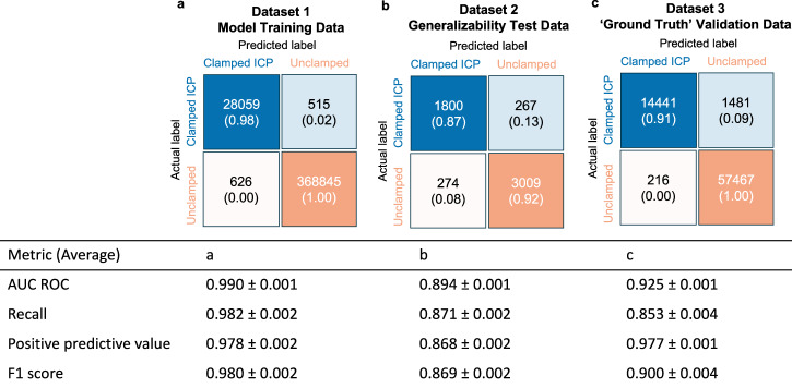
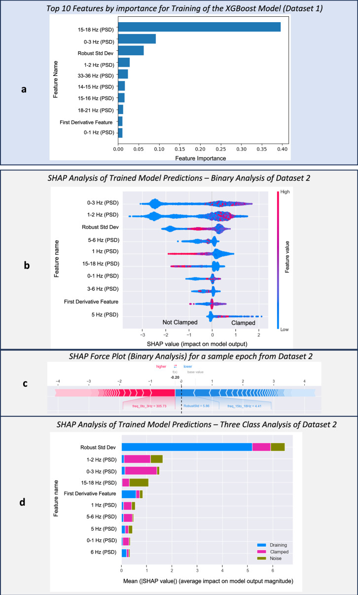
Patients with acute brain injuries are at risk for life threatening elevated intracranial pressure (ICP). External Ventricular Drains (EVDs) are used to measure and treat ICP, which switch between clamped and draining configurations, with accurate ICP data only available during clamped periods. While traditional guidelines focus on mean ICP values, evolving evidence indicates other waveform features may hold prognostic value. However, current machine learning models using ICP waveforms exclude EVD data due to a lack of digital labels indicating the clamped state, markedly limiting their generalizability. We introduce, detail, and validate CICL (Classification of ICP epochs using a machine Learning framework), a semi-supervised approach to classify ICP segments from EVDs as clamped, draining, or noise. This paves the way for multiple applications, including generalizable ICP crisis prediction, potentially benefiting tens of thousands of patients annually and highlights an innovate methodology to label large high frequency physiological time series datasets.


Conflict of interest statement

Competing interests: The authors declare no competing financial or non-financial interests that have a relationship to this work as defined by Nature Portfolio. The authors declare the following non-competing disclosures: Vishank Shah disclosures: VS received honoraria (<1000$) from Astra Zeneca and serves on the Editorial Board for Neurohospitalist. Sudha Yellapantula works as a Researcher for Medical Informatics Corp (MIC, Houston TX) and reports no competing interests. MIC is a company that provides the Sickbay platform to various hospitals, for clinical and research use of the data. Medical Informatics provided no funding and/or support for the study. Jose I Suarez disclosures: ex-officio member of the Board of Directors of the Neurocritical Care Society; member of the Scientific Advisory Board for Cyban; Member of the Data Safety Monitoring Board for clinical trials sponsored by Acasti and Perfuze; member of the Advisory Board for AstraZeneca for Andexxa Medical Strategy. Susanne Muehlschlegel disclosures: ex-officio member of the Board of Directors of the Neurocritical Care Society; Consultant for Acasti Pharma as a member of the clinical endpoint adjudication committee. Has received speaking and writing honoraria from the American Academy of Neurology. Serves on the Editorial Board for Neurocritical Care and Stroke (unpaid).

Figures

Fig. 1
Fig. 1. EVD functionality and stop-cock mechanism with waveform output.
The figure illustrates an external ventricular drain (EVD) surgically inserted into a patient’s intracranial ventricular system. The EVD comprises several key components, including a flexible catheter that connects the brain’s ventricles to an external drainage system. This system features a graduated collection chamber to measure cerebrospinal fluid (CSF) volume, a pressure transducer for monitoring intracranial pressure (ICP), and a leveling device to ensure accurate alignment with the patient’s head for precise readings. A critical element of the EVD system is the three-way stopcock, a small valve with three ports and a rotatable valve (red) that controls CSF flow. When the stopcock is in position B (clamped), CSF flows from the ventricles to the pressure transducer only, allowing for accurate ICP waveform measurement without drainage. In positions A or C (draining), CSF flows from the ventricles to the collection chamber, generating an inaccurate ICP waveform at the transducer. Position D, rarely used, results in clamping without ICP waveform generation as the CSF bypasses the transducer. At regular intervals established by unit protocols, a critical care nurse rotates the stopcock valve to position A to clamp the EVD, levels the system at a specific height relative to the patient’s head (usually at the external auditory meatus level, approximating the foramen of Monro), and collects 30 s to 2 min of accurate ICP waveform data. The nurse also records and empties the collected CSF before reopening the EVD to drain by moving the valve to position B or C. The waveform on the left of the figure shows a typical clamped and accurate ICP waveform. This waveform generally consists of three peaks: P1 (percussive wave), P2 (tidal wave), and P3 (dicrotic wave). P1 is generated by arterial pulsations, P2 reflects intracranial compliance, and P3 corresponds to the closure of the aortic valve. The P2/P1 ratio is a well-established indicator of intracranial compliance.
Fig. 2
Fig. 2. Box plot of mean ICP values for each dataset.
A box plot of mean ICP values for each dataset, with the red crosses showing average mean ICP value and the lines inside boxes showing median value. The lines at top of figure denote statistical significance between any two datasets. The presence of *** above the lines indicates significant differences (alpha value 0.05, p value extremely close to zero) in the mean ICP values among the datasets. The pairwise comparison was conducted using the Wilcoxon rank-sum test, as the datasets do not follow a normal distribution, necessitating a non-parametric alternative, and they differ in size. It is shown that all three datasets have significantly different distribution, underscoring and validating the model’s ability to generalize to unseen dataset with different mean ICP distribution.
Fig. 3
Fig. 3. Performance comparison of XGBoost model with different feature sets.
This plot shows the performance of the XGBoost model using different feature sets - and it was found that the expanded feature space improved the generalizability test results. It is interesting to note that the model performance on dataset 1 (10 fold CV test set) remains almost constant. However, performance in generalizing to dataset 2 improves significantly with increasing the number of features. This suggests that the model is robust and consistent in its prediction within the training set. The improvement in generalization performance highlights the importance of feature quality and relevance, and that inclusion of more informative features do boost the model’s ability to generalize.
Fig. 4
Fig. 4. Confusion matrices and model performances across three datasets.
This figure shows the confusion matrices on the outputs of the model on each Dataset to demonstrate model performance. a Dataset 1 - model training data performance using 10-fold stratified cross-validation b Trained model performance on dataset 2 - generalizability test data c Trained model performance on dataset 3 - `ground truth' validation data. A number following the ` ± ' symbol represents the standard deviation (s.d.) across 10 folds for (a) and the standard error of the mean (s.e.m.) for (b, c).
Fig. 5
Fig. 5. Model feature importance and SHAP analysis on model output.
This figure provides information about the features indentified as important by the model, as well as SHAP analysis of the outputs of the model. a Model feature importance plot. Top 10 most important features identified by the model, plotted in descending order of importance. The feature at the top of the chart represents the most significant contributor to the model’s predictions, with decreasing importance observed for the subsequent features. b The SHAP summary plot for binary-class evaluation. The y-axis list features that have the highest contribution to SHAP value in descending order of importance. Each dot on the plot represents a single epoch, with the color indicating the feature value --- blue for lower values and red for higher values, as shown on the color bar. The SHAP values on the x-axis measure each feature’s impact on the model’s prediction, where positive SHAP values (towards the right) indicate a feature’s contribution to classifying a segment as “Clamped,” and negative SHAP values (towards the left) suggest a contribution to the “Not Clamped” classification. c The SHAP force plot. This figure shows features' impact on model output for a sample epoch. Only the top contributors are displayed, while less important contributions are represented by smaller stacked arrows. The direction of arrows indicate the force of pushing toward a certain (positive or negative) model prediction. d The SHAP summary plot for multi-class evaluation. Top 10 features having highest average impact on model output magnitude for all three classes (clamped, draining and noise), identified by the model, plotted in descending order of importance. The feature at the top of the chart represents the most significant contributor (on average) to the model’s predictions.
Fig. 6
Fig. 6. CICL framework in action.
A visualization of testing data from a single day for seven individual patients. The waveform is color-coded based on the corresponding CICL classification label, with a gray vertical line (ag) marking specific region in the waveform where a zoomed-in 5-second segment and its mean values are observed. This visualization reveals valid clamped ICP data, including negative values. Additionally, the same waveform shape can occur at different scales, highlighting the variability in ICP waveform patterns across the dataset.
Fig. 7
Fig. 7. Summary of methods.
Each panel of the figure provides a summary of a key step in the overall methodology of the paper. a ICP waveform data from all three datasets underwent cleaning to remove outliers, correct inaccuracies, and handle missing values. The cleaned data was segmented into “epochs” using an established change-point detection tool with parallel processing of the segments. b Dataset 1 served as the training dataset. An initial set of seven features was extracted for each epoch in this dataset. Using unsupervised k-means clustering, these epochs were grouped into 100 clusters based on the extracted features. A neurointensivist manually labeled a large number of epochs using a rigorous sampling methodology which providing labeled data for model training. These epochs were then split into a train/test split. A grid search with 5-fold cross validation was used to optimize parameters. We used these labeled epochs, with the initial seven features, to train and compare six different supervised machine learning methods based on performance and accuracy. The best performing model, in this case XGBoost, was identified. To train the final model, an expanded set of 383 features was then extracted for each of the labeled epochs. These features were used to train an XGBoost model to develop CICL, our trained model. c Dataset 2 was used to evaluate the performance of the trained model. The same 383 features were generated for all epochs in Dataset 2, and the trained model produced labels for these epochs. To determine accuracy, a subset of Dataset 2 epochs was manually labeled by a neurointensivist, and the model’s labels were compared with these manual labels. d Dataset 3 was prospectively collected with real-time ground-truth labeling of clamping, draining, and noise generation by a trained clinical observer at the bedside during data recording. The same set of 383 features was extracted for each epoch, and the trained model generated labels for comparison against the ground-truth labels to assess performance and accuracy e Multi-class Classification: An example of the model output for clamped, draining, and noise epochs.
Fig. 8
Fig. 8. Overview of the labeling pipeline.
This figure showcases the methodology used for labeling of the PELT segmented epochs. These labels were later used to train the models. In this figure, D, C, and N refer to “draining EVD,” “clamped ICP,” and “noise,” respectively. Following change point detection and k-means++ clustering, data epochs are grouped into 100 clusters. For each cluster, the pipeline performs two key steps: (1) Rapid Labeling: If 98% of the epochs within a cluster meet the criterion of having a standard deviation <0.75, the entire cluster is classified as `draining EVD'. Otherwise, the pipeline proceeds with further labeling steps. In the training data, ≈70– 80% of the epochs per EVD recording were rapidly labeled using this threshold, found by hours of manual verification. (2) Cluster Categorization: Clusters are categorized based on size. The top 10 largest clusters are labeled as `large clusters', clusters with fewer than 100 epochs are labeled as `small clusters', and the remaining clusters are labeled as `mid-size clusters'. Each category undergoes a specific sampling process as illustrated in the figure. (3) Label Propagation: The sampled data are then labeled by a single neurointensivist, with labels propagated back to the entire cluster based on label homogeneity. The propagated data are marked as `labeled and verified'. The label homogeneity is determined by the percentage of epochs within a cluster that share the same label, with specific criteria for each label as depicted in the figure. If label homogeneity does not satisfy requirement, propagation does not occur and data stays `unverified' and thus not used in data training and testing. Overall, the neurointensivist manually labeled 3.6% of all epochs in dataset 1, which resulted in a total of 85.15% of labeled epochs (after threshold labeling and propagated labels).

Similar articles

References

    1. Le Roux, P. et al. Consensus summary statement of the international multidisciplinary consensus conference on multimodality monitoring in neurocritical care: a statement for healthcare professionals from the neurocritical care society and the european society of intensive care medicine. Neurocritical Care21, 1–26 (2014). - PMC - PubMed
    1. Carney, N. et al. Guidelines for the management of severe traumatic brain injury. Neurosurgery80, 6–15 (2017). - PubMed
    1. Stocchetti, N. & Maas, A. I. Traumatic intracranial hypertension. N. Engl. J. Med.370, 2121–2130 (2014). - PubMed
    1. Rosner, M. J. & Becker, D. P. Origin and evolution of plateau waves: experimental observations and a theoretical model. J. Neurosurg.60, 312–324 (1984). - PubMed
    1. Robba, C. et al. Intracranial pressure monitoring in patients with acute brain injury in the intensive care unit (synapse-icu): an international, prospective observational cohort study. Lancet Neurol.20, 548–558 (2021). - PubMed

LinkOut - more resources