FREQ-NESS Reveals the Dynamic Reconfiguration of Frequency-Resolved Brain Networks During Auditory Stimulation

Abstract

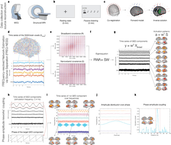
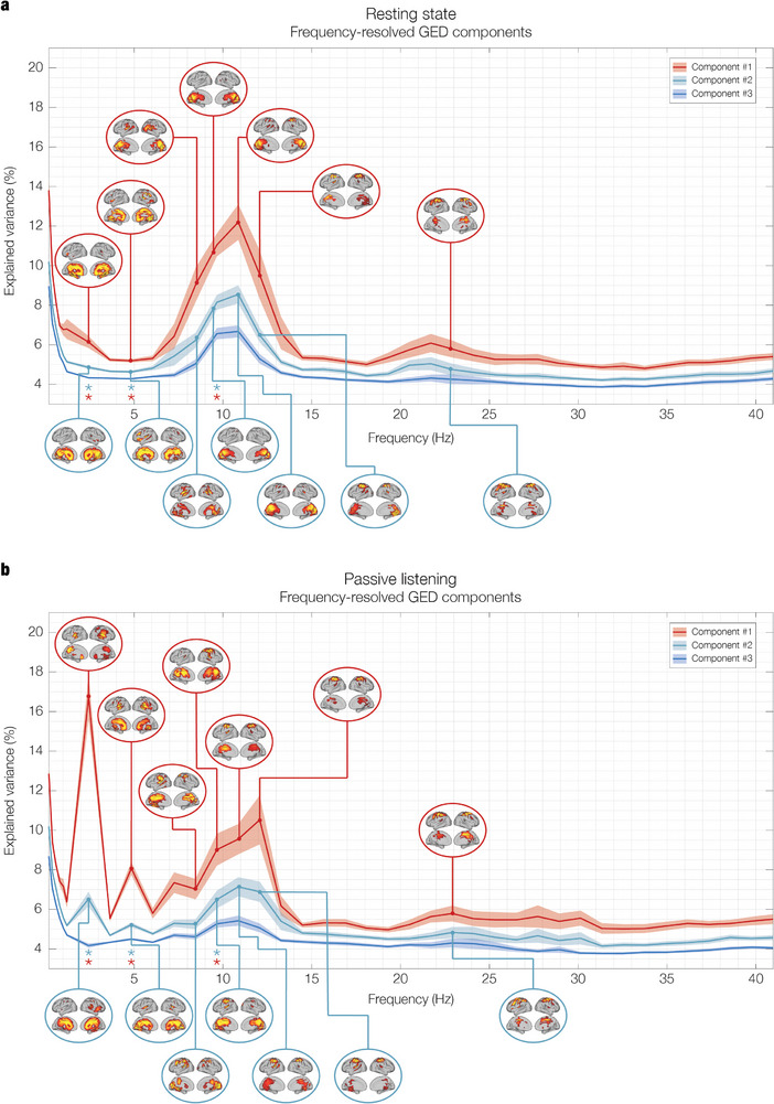
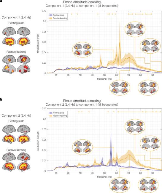
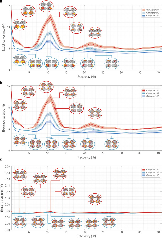
The brain is a dynamic system whose network organization is often studied by focusing on specific frequency bands or anatomical regions, leading to fragmented insights, or by employing complex and elaborate methods that hinder straightforward interpretations. To address this issue, a new analytical pipeline named FREQuency-resolved Network Estimation via Source Separation (FREQ-NESS) is introduced. This pipeline is designed to estimate the activation and spatial configuration of simultaneous brain networks across frequencies by analyzing the frequency-resolved multivariate covariance between whole-brain voxel time series. In this study, FREQ-NESS is applied to source-reconstructed magnetoencephalography (MEG) data during resting state and isochronous auditory stimulation. Our results reveal simultaneous, frequency-specific brain networks during resting state, such as the default mode, alpha-band, and motor-beta networks. During auditory stimulation, FREQ-NESS detects: 1) emergence of networks attuned to the stimulation frequency, 2) spatial reorganization of existing networks, such as alpha-band networks shifting from occipital to sensorimotor areas, 3) stability of networks unaffected by auditory stimuli. Furthermore, auditory stimulation significantly enhances cross-frequency coupling, with the phase of auditory networks attuned to the stimulation modulating gamma band amplitude in medial temporal lobe networks. In conclusion, FREQ-NESS effectively maps the brain's spatiotemporal dynamics, providing a comprehensive view of brain function by revealing a landscape of simultaneous, frequency-resolved networks and their interaction.

Keywords: auditory processing; brain networks; cross‐frequency coupling (CFC); generalized eigendecomposition (GED); magnetoencephalography (MEG); resting state.

Figure 1

FREQuency‐resolved network estimation via source separation (FREQ‐NESS). The figure provides an overview of the FREQ‐NESS analytical pipeline. a) MEG was used to collect neurophysiological data in the experimental conditions, while structural MRI was acquired in a separate session. b) Participants underwent MEG recordings during two experimental conditions: 5 min of resting state (RS) and 5 min of passive listening (PL) to isochronous auditory tone sequence at a rate of 2.4 Hz. c) To compute MEG source reconstruction, we performed co‐registration between MEG data and individual MRI anatomical scans, forward model (single shell), and inverse solution using beamforming. d) The source reconstruction generated one time series for each of the 3559 brain voxels from an 8‐mm grid parcellation of the brain. e) The covariance matrices R and S were computed from the broadband voxel data matrix (R) and from the narrowband filtered voxel data matrix (S); the procedure was repeated for a sample of 86 frequencies, computing a new S covariance matrix upon each iteration. f) Generalized eigendecomposition (GED) was computed by solving the eigenequation RWΛ = SW for the eigenvectors (W) to find the weighted combinations of brain voxels to separate frequency‐specific networks; the associated eigenvalues (Λ) express the amount of variance explained by each network component. g) Network activation time series and spatial patterns were computed. The spatial filters (w) were applied to the broadband voxel data matrix (X_broad) via matrix multiplication to reconstruct its components (y) as network activation time series; the same spatial filters were applied to the narrowband covariance matrix S to compute the spatial activation patterns (a) as the components’ projections in voxel space. h) The phase of the bandpass filtered time series of the 2.4 Hz components of interest (brain networks) is extracted via Hilbert transform for subsequent cross‐frequency coupling (CFC) analysis. i) To investigate the modulation of network interactions (phase of the 2.4 Hz brain networks modulating the amplitude over all the frequency bins), the modulation of frequency‐specific brain networks as a function of the low‐frequency modulating network was quantified as amplitude modulation. j) For each network, mean power values were calculated for all the phase bins, resulting in an amplitude distribution over the 2.4 Hz network's phase. k) For each frequency‐specific network, an index of modulation strength was computed by fitting a sinewave to the modulation curves and computing its amplitude; this enabled the identification of significant interactions across networks operating at specific frequencies (here, the phase of the 2.4 Hz brain networks modulating the amplitude over the higher frequency bins).

Figure 2

Network landscape: eigenspectrum and spatial activation patterns during a) resting state (RS) and b) passive listening (PL). The first element of the network landscape is the eigenspectrum, which consists of the eigenvalues expressing the percentage of variance explained by the associated GED components, plotted over the frequencies. The solid lines represent the mean normalized eigenvalues averaged across 26 participants (N = 26), with shaded areas indicating the standard error of the mean (SEM). Stars denote frequency bins where significant differences were detected using a two‐tailed signed‐rank Wilcoxon test, following FDR correction for multiple comparisons. The second element displays the spatial activation patterns associated with the top GED components for the frequencies exhibiting the highest explained variance. Each pattern highlights the extent of each brain voxel's contribution to the respective network. To improve visualization, the eigenspectra are shown here for the first three GED components (sorted by explained variance) over a portion of the frequency spectrum (0.2 to 40.9 Hz), while the topographies of the first two components are shown for the frequencies with the highest explained variance. For an extended version of the network landscape, see Figure S1 (Supporting Information). a) RS: The network landscape reveals a 1/f exponential decay of explained variance in the low delta range and local maxima in the alpha (10.9 Hz) and beta (22.9 Hz) frequency ranges. The spatial activation patterns show the typical topographies expected from the brain at rest, namely the broad mesial distribution associated with the DMN for low frequencies not engaged in stimulus processing (2.4 and 4.8 Hz), parieto‐occipital distribution for the alpha network (10.9 Hz), and sensorimotor involvement for the beta network (22.9 Hz). Notably, while frequencies on the left side of the alpha peak exhibit parieto‐occipital activation (8.4 and 9.6 Hz), the higher end of the range is characterized by sensorimotor activation (12.1 Hz). In the beta range, the explained variance peaks at 22.9 Hz, and the spatial pattern shows activation limited to sensorimotor regions. b) PL: Significant reorganization of brain networks occurs in response to auditory stimulation. The eigenspectrum exhibits a pronounced peak at the stimulation frequency of 2.4 Hz and its first harmonic at 4.8 Hz, reflecting the emergence of brain networks attuned to the rhythmic auditory stimulus. The spatial activation patterns at 2.4 Hz show focal engagement of the right auditory cortex, particularly in Heschl's gyrus, with additional involvement of broader medial temporal regions in the 4.8 Hz component, indicative of secondary auditory processing. Another key change observed in this condition is the shift in the alpha peak from 10.9 Hz in the resting state to 12.1 Hz during listening, accompanied by a posterior‐to‐anterior shift in spatial activation from parieto‐occipital to sensorimotor regions. This reorganization suggests that auditory stimulation induces a rearrangement of alpha networks, likely reflecting increased readiness for action and sensory processing in response to the rhythmic stimulus. The arrangement of beta remains stable across conditions, both in terms of eigenspectrum and spatial patterns.

Figure 3

Network landscape: cross‐frequency coupling during resting state (RS) and passive listening (PL). The figure shows the interaction between each of the two low‐frequency 2.4 Hz auditory networks and all the higher‐frequency networks during RS and PS. The plots display the modulation strength, a measure of how the phase of the low‐frequency network component modulates the amplitude of the other network components. The solid lines represent the mean modulation strength averaged across 26 participants (N = 26), with shaded areas indicating the standard error of the mean (SEM). Stars denote frequency bins where significant differences were detected using a right‐tailed signed‐rank Wilcoxon test, following FDR correction for multiple comparisons. a) Component #1 (2.4 Hz): The left panel shows the spatial activation patterns for component #1 at 2.4 Hz in both RS and LS. In RS, the activation is concentrated in medial temporal regions, including the hippocampus, while during listening, it shifts toward primary auditory areas, particularly Heschl's gyrus, indicating the auditory network's engagement with the rhythmic stimulus. The right panel displays the phase‐amplitude coupling (PAC) results, showing significant modulation of high gamma band activity (70–90 Hz) by the 2.4 Hz component during listening. This modulation is notably stronger than in the resting state, suggesting enhanced cross‐frequency coupling driven by auditory processing. b) Component #2 (2.4 Hz): The left panel shows the spatial activation patterns for component #2 at 2.4 Hz, which involve a broader network during both conditions, including auditory and medial temporal regions. In PL, this component also recruits additional prefrontal regions, indicating a higher‐level integration of auditory information. The right panel shows that, similar to component #1, the modulation of gamma band activity by component #2 is significantly stronger during listening, particularly in the 60–80 Hz range, reinforcing the finding that auditory stimulation enhances the coupling between low‐frequency auditory rhythms and high‐frequency gamma oscillations. These results highlight the dynamic reconfiguration of cross‐frequency interactions between brain networks in response to auditory stimulation, with a clear enhancement of PAC between low‐frequency auditory networks and high‐frequency gamma networks. This result underscores that gamma oscillations play a key role in processing rhythmic auditory stimuli, mediated by the interaction with auditory networks attuned to the stimulation frequency.

Figure 4

Network landscape of randomized resting state (RS) data: eigenspectrum and spatial activation patterns. This figure illustrates the frequency‐resolved brain networks obtained using FREQ‐NESS applied to the original data, randomized with two different strategies. 1) Label randomization: The brain voxel indices were shuffled consistently across the entire time series, meaning the temporal data remained intact but was reassigned to different brain voxels; 2) Point‐wise label randomization: The voxel indices were shuffled independently for each time point, disrupting the temporal structure. As shown in Figure 2, the first element of the network landscape is the eigenspectrum, which shows the eigenvalues representing the percentage of variance explained by the GED components across frequencies. Solid lines denote the mean normalized eigenvalues across participants, with shaded areas indicating the standard error of the mean (SEM). The second element depicts spatial activation patterns associated with the top GED components at frequencies with the highest explained variance. Each pattern illustrates the contribution of each brain voxel to the corresponding network. For enhanced visualization, the eigenspectra are presented for the first three GED components (sorted by explained variance) across a frequency range of 0.2 to 40.9 Hz. The spatial topographies of the first two components are shown for frequencies with the highest explained variance. a) Original data: To allow an easier comparison, we report the same results for RS data shown in Figure 2. b) Randomization 1 (Labels) preserved the eigenspectrum but disrupted the spatial activation patterns, maintaining the frequency content and variance explained by GED components but yielding physiologically meaningless patterns. c) Randomization 2 (Point‐wise labels) disrupted both the eigenspectrum and spatial activation patterns, flattening the exponential decrease in variance explained by subsequent GED components. This suggests that reshuffling voxels for each time point disrupts the temporal structure of the signal and reduces the variance explained by GED components to ≈0.06% across frequencies, highlighting potential variance contributions attributable to chance. The solid lines represent the mean normalized eigenvalues averaged across 26 participants (N = 26), with shaded areas indicating the standard error of the mean (SEM). A two‐tailed signed‐rank Wilcoxon test was conducted separately for each randomization against the original data. Since Randomization 1 yielded no significant differences, while Randomization 2 showed significant differences across all frequency bins following FDR correction for multiple comparisons, statistical significance is not reported in the figure to avoid redundancy.

References

1. Deco G., Tononi G., Boly M., Kringelbach M. L., Nat. Rev. Neurosci. 2015, 16, 430. - PubMed
1. Deco G., Cabral J., Woolrich M. W., Stevner A. B. A., van Hartevelt T. J., Kringelbach M. L., Neuroimage 2017, 152, 538. - PMC - PubMed
1. Engel A. K., Gerloff C., Hilgetag C. C., Nolte G., Neuron 2013, 80, 867. - PubMed
1. Buzsáki G., Logothetis N., Singer W., Neuron 2013, 80, 751. - PMC - PubMed
1. Nobre A. C., van Ede F., Nat. Rev. Neurosci. 2018, 19, 34. - PubMed
LinkOut - more resources