Frequentist Grouped Weighted Quantile Sum Regression for Correlated Chemical Mixtures

Abstract

As individuals are exposed to a myriad of potentially harmful pollutants every day, it is important to determine which actors have the greatest influence on health outcomes. However, jointly modeling the associations of multiple pollutant exposures is often hindered by the presence of highly correlated chemicals originating from a common source. A popular approach to analyzing associations between a disease outcome and several highly correlated exposures is Weighted Quantile Sum Regression (WQSR) modeling. WQSR provides increased stability in estimating model parameters but requires data splitting to estimate individual and group effects of chemicals, which reduces the power of the approach. A recent Bayesian implementation of WQSR regression provides a model fitting procedure that avoids data splitting at the cost of high computational expense on large data. In this paper, we introduce a Frequentist Grouped Weighted Quantile Sum Regression (FGWQSR) model that can be fitted efficiently to large datasets without requiring data splitting. FGWQSR produces estimates of the joint effect of mixture groups and of individual chemicals, and likelihood-ratio-based tests that account for FGWQSR's non-standard asymptotics. We demonstrate that FGWQSR is well calibrated for type-I errors while outperforming both Bayesian Grouped Weighted Quantile Sum Regression and Quantile Logistic Regression in terms of statistical power to detect the effects of mixture groups and individual chemicals. In addition, we show that FGWQSR is robust to model misspecification and can be fitted on large datasets in a fraction of the time required for BGWQSR. We apply FGWQSR to a dataset of 317 767 mother-child pairs with exposure profiles generated by chemical transport models to study the associations between several components found in particulate matter with an aerodynamic diameter smaller than 2.5 $\mu m$ (PM ${}_{2.5}$ ) and child Autism Spectrum Disorder (ASD) diagnosis before age 5. PM ${}_{2.5}$ copper and PM ${}_{2.5}$ crustal material are found to be statistically significantly associated with ASD diagnosis by five years of age.

Keywords: autism spectrum disorder; chemical mixture modeling; constrained optimization; group sign constrained regression; non‐regular likelihood asymptotics; pollutant mixture modeling; weighted quantile sum regression.

FIGURE A1

Results of correctly specified simulations comparing the performance of FGWQSR, BGWQSR, and QLR over 1 000 replicates of simulated datasets with size $n=500$ with a case‐control ratio of approximately 1:1. Columns 1–4 correspond to mixture group effect power, single chemical power, individual chemical MSE, and individual chemical bias, respectively. In the presented simulations, CCS is fixed to (0.9,0.5) and the weight distribution of chemicals within groups is set as follows: ${\mathbf{w}}_A=(\frac{1}{3},\frac{1}{3},\frac{1}{3},0,0)$; ${\mathbf{w}}_B=(\frac{1}{2},\frac{1}{2},0,0)$; and ${\mathbf{w}}_C=(\frac{1}{3},\frac{1}{3},\frac{1}{3},0,0)$. Each row denoted (A)–(E) corresponds to five levels of SOA: ${\text{SOA}}_1=$(1, 1, 1); ${\text{SOA}}_2=$(0.9,1.1,1.1); ${\text{SOA}}_3=$(0.85, 1.15, 1.15); ${\text{SOA}}_4=$(0.8, 1.2, 1.2); and ${\text{SOA}}_5=$(0.7, 1.3, 1.3). Lines and points denoted by green, mustard, and light blue colors correspond to metrics computed from FGWQSR, BGWQSR, and QLR models, respectively. Dashed horizontal purple and black lines in power plots denote powers of 0.04, 0.05, and 0.06 as a reference for type 1 errors in the presence of null mixture group effects and null individual chemicals effects. Individual chemical effects colored in dark red denote null individual chemicals with weights of 0. Note that row (A) corresponds to the case where all group effects are null, which imposes that all individual chemical effects are also null.

FIGURE A2

Results of moderate misspecification simulations comparing the performance of FGWQSR, BGWQSR, and QLR over 1 000 replicates of simulated datasets with size $n=500$ with a case‐control ratio of approximately 1:1. Columns 1–4 correspond to mixture group effect power, individual chemical power, individual chemical MSE, and individual chemical bias, respectively. In the presented simulations, CCS is fixed to (0.9,0.5) and the weight distribution of chemicals within groups is set as follows: ${\mathbf{w}}_A=(\frac{1}{3},\frac{1}{3},\frac{1}{3},0,0)$; ${\mathbf{w}}_B=(\frac{1}{6},\frac{1}{6},\frac{1}{6},\frac{1}{6},-\frac{1}{6},-\frac{1}{6})$; and ${\mathbf{w}}_C=(\frac{1}{3},\frac{1}{3},\frac{1}{3},0,0)$. Each row denoted (A)–(E) corresponds to one of five levels of SOA: ${\text{SOA}}_1=$(1, 1, 1); ${\text{SOA}}_2=$(0.9, 1.1, 1.1); ${\text{SOA}}_3=$(0.85, 1.15, 1.15); ${\text{SOA}}_4=$(0.8, 1.2, 1.2); and ${\text{SOA}}_5=$(0.7, 1.3, 1.3). Lines and points denoted by green, mustard, and light blue colors correspond to metrics computed from FGWQSR, BGWQSR, and QLR models, respectively. Dashed horizontal purple and black lines in power plots denote powers of 0.04, 0.05, and 0.06 as a reference for type 1 errors in the presence of null mixture group effects and null individual chemicals effects. Individual chemical effects colored in dark red denote null individual chemicals with weights of 0. Individual chemicals in group B with a dark blue shading (B1–B4) have a positive weight of size $\frac{1}{6}$ while chemicals with an orange shading (B5 and B6) have a negative weight of size $-\frac{1}{6}$. Note that row (A) corresponds to the case where all group effects are null, which imposes that all individual chemical effects are also null.

FIGURE A3

Results of runtime comparison simulations between FGWQSR and BGWQSR. Runtimes are resolved at dataset sizes of $n$ = {100, 500, 1 000, 2 000, 5 000, 7 500, 10 000, 20 000, 50 000, 100 000} with a case‐control ratio of approximately 1:1, and CCS fixed to (0.7, 0.3). Simulations are run for 3‐group and 6‐group mixture configurations with ${\text{SOA}}_{\text{3‐group}}$ = (0.8, 1, 1.2) and ${\text{SOA}}_{\text{6‐group}}$ = (0.8, 1, 1.2, 0.8, 1, 1.2) with weight distributions as follows: ${\mathbf{w}}_1=(\frac{1}{3},\frac{1}{3},\frac{1}{3},0,0)$, ${\mathbf{w}}_2=(\frac{1}{2},\frac{1}{2},0,0)$, and ${\mathbf{w}}_3=(\frac{1}{3},\frac{1}{3},\frac{1}{3},0,0)$; ${\mathbf{w}}_1=(\frac{1}{3},\frac{1}{3},\frac{1}{3},0,0)$, ${\mathbf{w}}_2=(\frac{1}{2},\frac{1}{2},0,0)$, and ${\mathbf{w}}_3=(\frac{1}{3},\frac{1}{3},\frac{1}{3},0,0)$, ${\mathbf{w}}_4=(\frac{1}{3},\frac{1}{3},\frac{1}{3},0,0)$, ${\mathbf{w}}_5=(\frac{1}{2},\frac{1}{2},0,0)$, and ${\mathbf{w}}_6=(\frac{1}{3},\frac{1}{3},\frac{1}{3},0,0)$. Lines and points denoted by green and orange colors correspond to the averaged runtimes of FGWQSR and BGWQSR models, respectively, over 10 replicates. Solid lines correspond to runtime simulations under a 3‐group configuration, while two‐dash lines correspond to runtime simulations under a 6‐group configuration. Model runtimes are plotted in the scale of ${\log }_{60}$(minutes) with labels at selected runtimes.

FIGURE A4

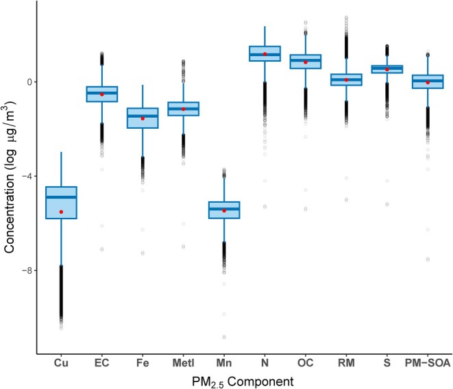
Distribution of pregnancy averaged PM component exposure generated from Source Oriented Chemical Transport models. Red points denote mean PM component exposure levels. Pollutant concentrations are displayed in $\log (\mu g/m^3)$ units.

FIGURE A5

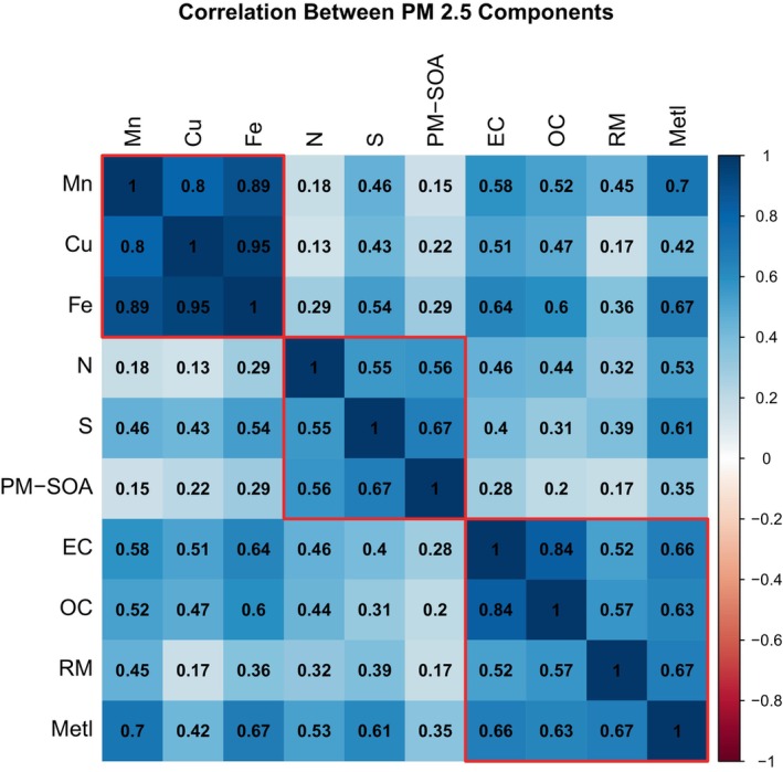
Correlation plot of PM components. Red boxes denote resulting clusters from hierarchical clustering on $1-C$, where $C$ denotes the correlation matrix, using a complete linkage and a cutpoint value to establish 3 clusters.