Dynamic ice-ocean pathways along the Transpolar Drift amplify the dispersal of Siberian matter

Abstract

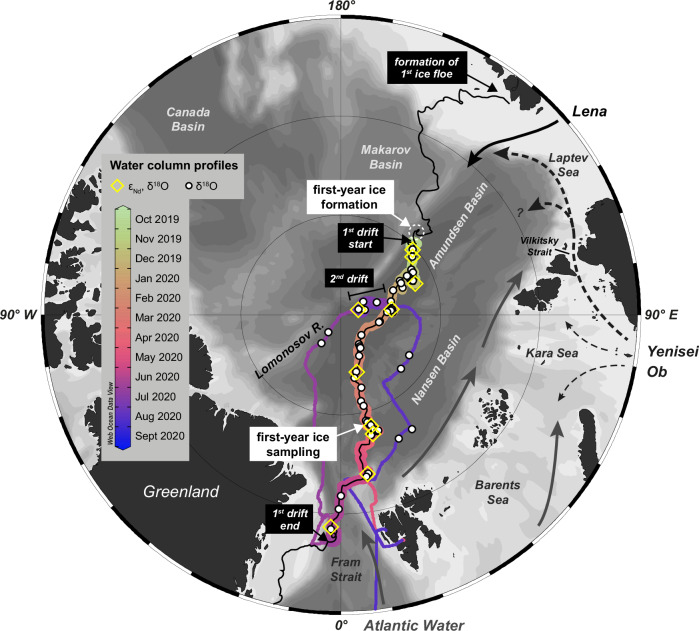
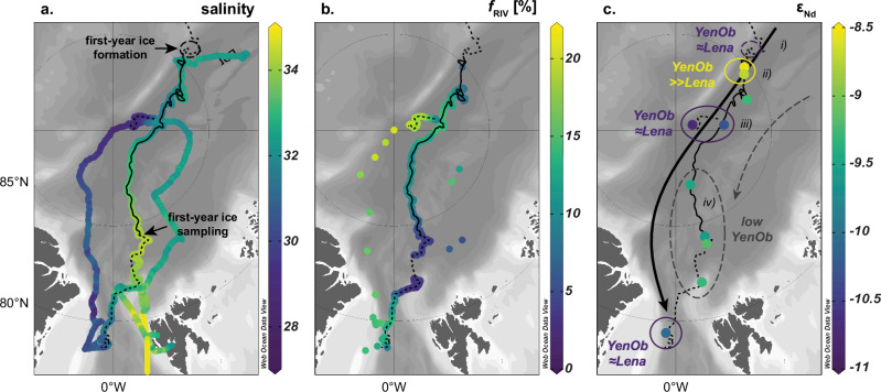
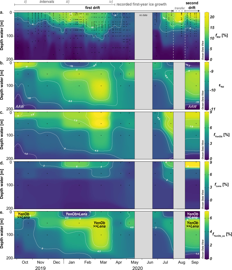
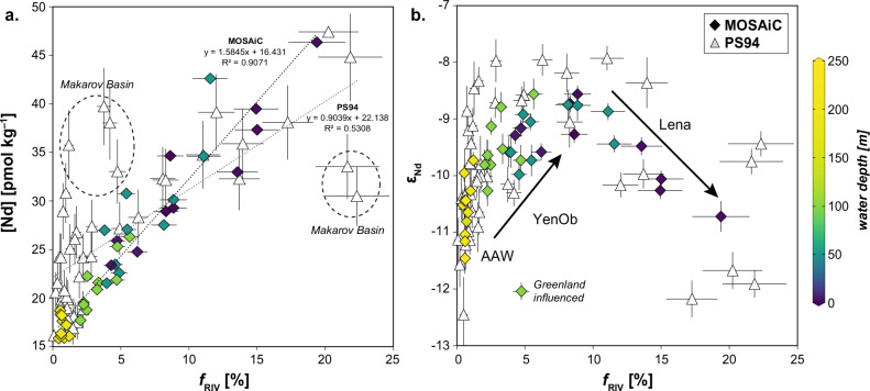
The Transpolar Drift (TPD) plays a crucial role in regulating Arctic climate and ecosystems by transporting fresh water and key substances, such as terrestrial nutrients and pollutants, from the Siberian Shelf across the Arctic Ocean to the North Atlantic. However, year-round observations of the TPD remain scarce, creating significant knowledge gaps regarding the influence of sea ice drift and ocean surface circulation on the transport pathways of Siberian fresh water and associated matter. Using geochemical provenance tracer data collected over a complete seasonal cycle, our study reveals substantial spatiotemporal variability in the dispersal pathways of Siberian matter along the TPD. This variability reflects dynamic shifts in contributions of individual Siberian rivers as they integrate into a large-scale current system, followed by their rapid and extensive redistribution through a combination of seasonal ice-ocean exchanges and divergent ice drift. These findings emphasize the complexity of Arctic ice-ocean transport pathways and highlight the challenges of forecasting their dynamics in light of anticipated changes in sea ice extent, river discharge, and surface circulation patterns.

Fig. 1. Map of the MOSAiC expedition drift tracks and locations of provenance tracer sampling.

The paths of the 1st and 2nd drifts (depicted by thick lines) and the transfers between them (shown as thin lines) are color-coded by date. In addition to water column stations, the start and end points of both drifts and the areas of first-year ice formation and sampling are highlighted. Since the exact location of first-year ice formation is unknown, a dashed white circle marks the drift interval during which first-year ice formation likely occurred (see main text for more information). The trajectory of the 1^st ice floe, both prior to the start of the 1st MOSAiC drift in October 2019 and after its conclusion in September 2020, is depicted by a thin, continuous black line. The source region of this ice floe is also marked. The approximate advective freshwater pathways on the Siberian Shelf are represented by a solid black arrow for the input from the Lena river and by several dashed black arrows for the contributions from the Yenisei and Ob rivers. The inflow of Atlantic Water through Fram Strait and the Barents Sea, and its subsequent route along the Arctic boundary current are indicated by solid grey arrows. The map was created using ODV and modified manually.

Fig. 2. Surface distribution of salinity, river water fraction and neodymium isotopes along the TPD.

a Continuous salinity measurements taken at 11 m depth using two thermosalinographs (SBE21, SeaBird GmbH) on board the RV Polarstern during both drifts and transit to and from the second ice floe^–. b River water content (f_RIV) in percent derived from the extensive stable oxygen isotope datasets^,. c Seawater neodymium isotope composition (ε_Nd), with major compositional trends depicted by colored circles that reflect the relative proportions of the two riverine endmembers Lena and Yenisei/Ob (YenOb > >Lena: pronounced excess of Yenisei/Ob water compared to Lena water; YenOb≈Lena: nearly equal contributions of these endmembers; see also Figs. 3e and 4b for interpretation). The dashed black circle in (a) marks the formation region of first-year ice, for which no seawater data are available. However, river water composition in this region, indicated in (c), is inferred from the first-year ice data. The pathway of the freshwater-rich Transpolar Drift, showing fluctuating river water contributions, is represented by a thick, solid black arrow in (c), while the advection of low amounts of Yenisei/Ob water along the Nansen Basin, likely exported from the northwestern Laptev Sea, is shown in the same map with a dashed grey arrow and a grey dashed circle around relevant stations. The drift tracks of the ice floes are shown as dashed black lines in all maps, while the recorded growth and drift of first-year ice are represented by a solid black line. The intervals i)–iv) shown in c correspond to major trends in river water proportions in the sea ice. The maps were created using ODV and modified manually.

Fig. 3. Evolution of provenance tracer parameters in the upper water column along the MOSAiC drift track.

a River water content (f_RIV, in percent) derived from the extensive stable oxygen isotope (δ¹⁸O) dataset (original salinity and δ¹⁸O data are shown in Supplementary Fig. S1). b Seawater neodymium isotope composition (ε_Nd) (corresponding neodymium concentrations shown in Supplementary Fig. S1). c Contributions of the Yenisei and Ob rivers (f_YenOb, in percent). d Contributions of the Lena river (f_Lena, in percent). e Excess of Yenisei/Ob river water relative to that of the Lena river (f_{YenOb_ex}, in percent), with marked zones of a pronounced excess of Yenisei/Ob water over Lena water (YenOb > >Lena) and nearly equal contributions of these endmembers (YenOb≈Lena). The grey line indicates recorded first-year ice growth along the drift, with an approximate temporal assignment of sea ice intervals ii)–iv). Grey areas indicate transit periods when the RV Polarstern traversed between ice floes and land, resulting in no data collection except for δ¹⁸O at two stations with shallow sampling during transit to the 2^nd ice floe (see Fig. 1). The sections were created using ODV and modified manually.

Fig. 4. Comparison between provenance tracer data obtained from the MOSAiC drift and the PS94 cruise (GEOTRACES transect GN04, 2015).

a River water content (f_RIV, in percent) derived from the three-component analysis plotted against neodymium concentration ([Nd], in pmol kg^–1). b River water fraction plotted against neodymium isotope composition (ε_Nd). Error bars for ε_Nd and [Nd] represent ± 2 standard deviations from measurements, while those for f_RIV account for both measurement errors and endmember variability. Black arrows indicate admixture of individual riverine Nd sources (Lena, YenOb) to Arctic Atlantic Water (AAW). PS94 cruise samples collected in the Makarov Basin, outside the freshwater-rich part of the Transpolar Drift, are highlighted with dashed circles. One MOSAiC sample from the Fram Strait, influenced by unradiogenic ε_Nd from Greenland (Supplementary Text 2), deviates from the data envelope in the f_RIV-ε_Nd space and is excluded from our analysis. MOSAiC data symbols are color-coded by sampling depth.

Fig. 5. Comparison between first-year ice profiles (upper x-axes) and surface seawater composition^,, (lower x-axes).

a Salinity (bulk salinity for sea ice). b Stable oxygen isotope compositions (δ¹⁸O). c Neodymium isotope compositions (ε_Nd). d Neodymium concentrations ([Nd]), and e Post-Archean Australian Shale normalized heavy-to-light rare earth element ratios (HREE/LREE). The first-year ice, recovered on April 8, 2020, is represented by tracer profiles derived from nine individual ice cores, with depth horizons merged to generate the presented data. In contrast, surface seawater data were collected throughout the ice growth and drift period but are plotted in the first-year ice profiles at ice core depths corresponding to the seawater sampling dates. These depths were calculated using an age model for the sea ice (‘Methods’). The sea ice composition is depicted by black lines, representing average values across varying depth segments, with grey fields indicating 2 standard deviations from measurements. Surface seawater composition, sampled at depths of 2 to 5 m, is represented by color-coded diamonds indicating the sampling date. For the upper 40 cm, where seawater data are unavailable, black diamonds denote low-salinity surface waters in August/September 2020 near the North Pole. Dark grey fields in (c and e) for the latter and x-axis error bars for the other seawater data represent 2 standard deviations from measurements for the ε_Nd and HREE/LREE values. Y-axis error bars on seawater data indicate ice age uncertainty. In panel (c), a color-coded line represents the ice core depth interval corresponding to ice drift when surface seawater salinities were below 32 (December 12, 2019, to February 10, 2020). Depth ranges for the four distinct sea ice intervals i)–iv) are indicated in the δ¹⁸O profile in (b). Differences in absolute values between sea ice and seawater composition arise from brine rejection for salinity, [Nd] and HREE/LREE ratios, and from fractionation during sea ice formation for δ¹⁸O.

Fig. 6. Relationship between individual riverine contributions in surface seawater and sea ice.

a Distribution of the percentage contributions of Lena and Yenisei/Ob rivers (Lena, YenOb) within the sea ice profile and their link to surface seawater values. The latter are represented by color-coded and black diamonds that indicate sampling dates, following the same scheme as in Fig. 5. The total riverine contribution in sea ice (‘total’ = f_Lena + f_YenOb) closely corresponds to f_RIV determined for surface seawater samples via the three-component analysis. b Comparison of the percentage contributions from the two riverine endmembers to surface seawater (diamonds) and sea ice (circles). Symbols are color-coded to represent sampling depth. Error bars in (a, b) represent uncertainties in water mass assessment related to measurement inaccuracies and endmember variability, except for y-axis error bars on seawater data in (a), which represent ice age uncertainty.

Fig. 7. Schematic comparison illustrating contrasting perspectives on TPD ice–ocean connectivity and ocean surface variability as primary drivers of matter redistribution.

a Simplified present perspective: This often implicitly adopted view stems from a limited understanding based on isolated assessments of ice and ocean reservoirs and their governing mechanisms. It emphasizes direct transport of matter from the Siberian Shelf to the Fram Strait or the Canadian Arctic Archipelago. In this representation, the Transpolar Drift (TPD) is depicted as a largely continuous pathway where a relatively homogeneous mix of Siberian river water (RW) and associated matter (rw) flows across the Arctic Ocean, both in the water column and within sea ice. The matter gradually blends with Atlantic-derived water (AW) and its constituents (aw), following a straightforward route. This approach concentrates on the bulk transfer of Siberian matter, with minimal differentiation among source contributions along the path. b Emerging perspective: While the transport mechanisms depicted in the simplified view remain valid, this perspective from our study emphasizes the dynamic and intricate nature of non-linear matter transport along the TPD. It highlights the variability in surface water composition and complex ice–ocean interactions. In this view, distinct matter mixtures (rm₁, rm₂) associated with various Siberian river waters (RW₁, RW₂), and additional sources, such as Greenlandic meltwater constituents (g) from Greenland (G), actively shape the composition of both seawater and sea ice at different points (l₁, l_x) and times (t₁, t_x) along the drift, with a future decrease in the long-range l₁t₁ pathway. The ice-driven redistribution of matter in the water column is indicated by white letters. Although both scenarios account for variable sea ice drift, straight arrows are used to provide a steady reference amidst surface layer fluctuations. Surface stresses are illustrated in (a) by arrows representing the Ekman spiral, alongside geostrophic flow, which together create an offset between ice drift and surface water flow. In (b), this offset becomes more pronounced as liquid freshwater transport is more constrained by geostrophic forcing, leading to a stronger decoupling between ice-driven and ocean-driven matter transport (represented by a dashed line).

References

1. Carmack, E. C. et al. Freshwater and its role in the Arctic Marine System: Sources, disposition, storage, export, and physical and biogeochemical consequences in the Arctic and global oceans. J. Geophys. Res. Biogeosci.121, 675–717 (2016).
1. Morison, J. et al. Changing Arctic Ocean freshwater pathways. Nature481, 66–70 (2012). - PubMed
1. Pfirman, S. L. et al. Potential for rapid transport of contaminants from the Kara Sea. Sci. Total Environ.202, 111–122 (1997). - PubMed
1. Rigor, I. G. & Colony, R. L. Sea-ice production and transport of pollutants in the Laptev Sea. Sci. Total Environ.202, 89–110 (1997). - PubMed
1. Peeken, I. et al. Arctic sea ice is an important temporal sink and means of transport for microplastic. Nat. Commun.9, 1505 (2018). - PMC - PubMed
LinkOut - more resources