Functionally distinct GABAergic amacrine cell types regulate spatiotemporal encoding in the mouse retina

Abstract

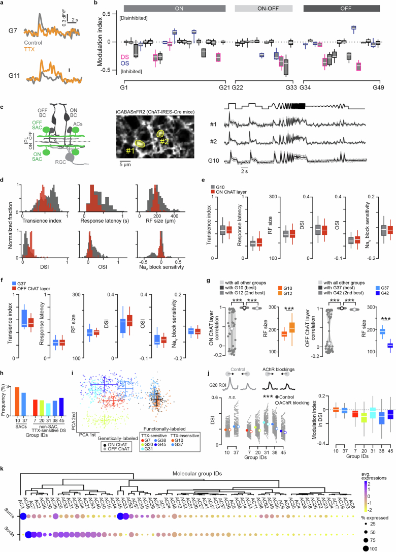
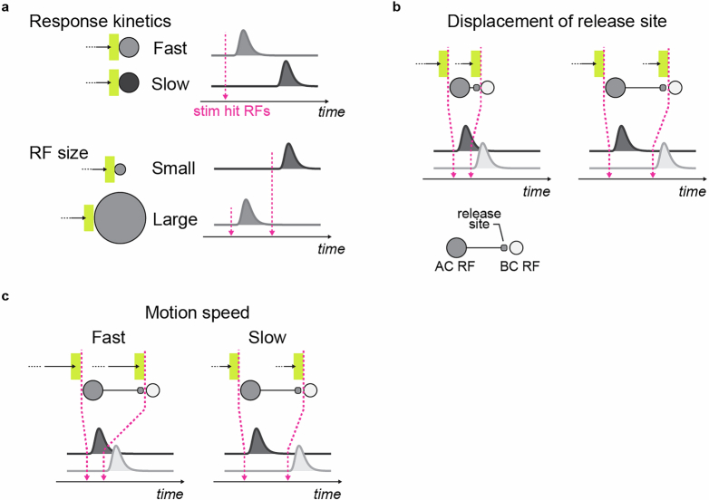
GABA (γ-aminobutyric acid) is the primary inhibitory neurotransmitter in the mammalian central nervous system. GABAergic neuronal types play important roles in neural processing and the etiology of neurological disorders; however, there is no comprehensive understanding of their functional diversity. Here we perform two-photon imaging of GABA release in the inner plexiform layer of male and female mice retinae (8-16 weeks old) using the GABA sensor iGABASnFR2. By applying varied light stimuli to isolated retinae, we reveal over 40 different GABA-releasing neuron types. Individual types show layer-specific visual encoding within inner plexiform layer sublayers. Synaptic input and output sites are aligned along specific retinal orientations. The combination of cell type-specific spatial structure and unique release kinetics enables inhibitory neurons to sculpt excitatory signals in response to a wide range of behaviorally relevant motion structures. Our findings emphasize the importance of functional diversity and intricate specialization of GABAergic neurons in the central nervous system.

Fig. 1. Functionally divergent GABA signal groups in the inner retinal layers.

a, Left: schematic of retinal neurons. AC, amacrine cell; BC, bipolar cell; SAC, starburst AC; RGC, retinal ganglion cell. Right: two-photon cross-sectional images of iGABASnFR2 and ChAT-IRES signals. L4 and L6 denote depths of OFF and ON ChAT processes, respectively. b, iGABASnFR2 (green) and ChAT-IRES (magenta) signals (7,098 ROIs, 11 retinae) in different imaging planes. The results were replicated 11 times independently. c, Dendrogram sorting of 49 identified GABA signal groups by direction/orientation selectivity and temporal dynamics (labels) (7,098 ROIs, 11 retinae). DS, direction selective (magenta); OS, orientation selective (blue); Sust., sustained; Trans., transient. d, Heatmap of ON response index (ON resp.), OFF response index (OFF resp.), bi-response index (Bi-resp.), transience index (Trans.) and latency index. e, Average static flash stimulus-evoked (left) and motion stimulus-evoked (right) signal for individual groups. Responses to a motion direction that produced maximum responses were temporally aligned relative to peak response timing and averaged. Gray shading indicates the s.d. Black line shows the average GABA signal for ROIs assigned to each group. f, Histogram of receptive field (RF) diameter for individual groups (color) and all groups (gray), each normalized to respective peaks. Source data

Fig. 2. Visual response properties of GABA signal groups.

a, Left: relationship between RF size and ON–OFF index for 49 groups (color coded). Circle size denotes fraction of recorded population. Right: relationship between contrast modulation and temporal frequency modulation indexes. b, Motion response properties: direction-selective index (DSI), orientation-selective index (OSI), motion/flash preference and speed tuning. dON, delayed ON. c, Heatmap, distribution of observed ROIs for 49 groups in layers between L2 and L8. Bars show the layer dominance index for each group (color coded). There were 7,098 ROIs and 11 retinae. Boxes represent 25th to 75th percentiles and median; whiskers represent 1.5 × interquartile range. Source data

Fig. 3. Intrinsic neural noise of GABA signals is consistent within each group.

a, Example ROIs of two different GABA signal groups (magenta and cyan). b, Noise correlation in four example pairs. c, Correlation matrix denoting three assemblies with intrinsic noise. d, RFs of ROIs in a using same color scheme. e, Comparison of distances between RF centers in assembled ROI pairs (cyan; 36 pairs, 1 retina) and others (gray; 192 pairs, 1 retina) used in a. P = 3.42 × 10⁻¹⁴; two-sided Mann–Whitney–Wilcoxon test. f, Relationship between ROI-to-ROI distances and noise correlation in ROI pairs in the same (blue; 4,373 pairs) and different (gray; 15,199 pairs) groups. There were 11 retinae. g, Matrix denoting frequency of GABA signal groups sharing significant neural noise. h, Dominance index for noise coincidence within the same group. Orange, groups with heterogeneous connections. ***P < 0.001; NS, not significant. Boxes represent 25th to 75th percentiles and median; whiskers represent 1.5 × interquartile range. Source data

Fig. 4. Direction-selective cell types.

a, DSI of ON (dark gray; 88 ROIs, P = 3.18 × 10⁻³⁴) and OFF (light gray; 62 ROIs, P = 3.58 × 10⁻³⁵) ChAT, non-DS groups (gray; 6,180 ROIs) and DS groups (color coded; 189 G10 ROIs, P = 1.74 × 10⁻⁸²; 148 G37, P = 2.64 × 10⁻⁵⁸; 133 G7, P = 6.38 × 10⁻⁵⁷; 128 G20, P = 2.11 × 10⁻⁶⁸; 109 G31, P = 3.71 × 10⁻⁷⁷; 129 G38, P = 3.14 × 10⁻⁸¹; 141 G45, P = 9.16 × 10^-47). ON and OFF ChAT targeted imaging, four retinae. Nontargeted imaging, 11 retinae. Kruskal–Wallis test, Bonferroni correction for multiple comparisons. b,c, Distributions of preferred directions in individual DS groups (b) and all TTX-sensitive DS groups (c). D, dorsal; T, temporal; V, ventral; N, nasal. d, Multidimensional features projected along the principal axes in datasets pooling functionally labeled (G10, G37, G7, G20, G31, G38 and G45) and genetically labeled (ON and OFF ChAT) DS groups (gray dots). Color-coded circles, average of each group. e, Top: similarity between functionally labeled and genetically labeled groups (11 retinae). Bottom: RF sizes (compared to G10: G7, P = 9.40 × 10⁻⁴³; G20, P = 3.22 × 10⁻⁷⁹; G31, P = 5.01 × 10⁻¹⁰⁴; G38, P = 5.53 × 10⁻²³; G45, P = 2.32 × 10⁻⁷⁸; compared to G37: G7, P = 2.88 × 10⁻²¹; G20, P = 2.90 × 10^-47; G31, P = 1.41 × 10⁻⁶⁷; G38, P = 7.99 × 10⁻⁹; G45, P = 9.28 × 10⁻⁴⁶). Kruskal–Wallis test, Bonferroni correction for multiple comparisons. f, Layer distribution of DS groups. g, Top: population of TTX-sensitive groups (left) and DS groups among them (right) in the functional clustering. Bottom: population of Na_V-expressing groups (left) and Na_V and acetylcholine receptor (AChR) coexpressing groups among them (right) in the molecular clustering. h, Expression of key neurotransmitter receptors in Na_V-expressing molecular groups. Groups expressing AChRs highlighted (pink, GABAergic; green, glycinergic). mGluR, metabotropic glutamate receptors; iGluR, ionotropic glutamate receptors; GlyR, glycine receptors; GABAR, GABA receptor; Markers, known amacrine cell type markers. Gene counts and metadata from Yan et al. (g,h). ***P < 0.001; boxes represent 25th to 75th percentiles and median; whiskers represent 1.5 × interquartile range. Source data

Fig. 5. Layer-specific inhibitory encoding of visual features.

a, Population of functionally characterized groups based on flash and motion responses. b, Fraction of significantly informative visual features encoded by specific groups. TF, temporal frequency. c, Profiles of visual encoding in 30 informative groups (Grps) sorted by Hotelling’s T² score. White diamonds show significantly informative features. d, Left: schematic of retinal layers. IPL sublayers denoted by light and dark gray. PR, photoreceptor; OPL, outer plexiform layer; INL, inner nuclear layer; GCL, ganglion cell layer. Right: fraction of significantly informative visual features for each IPL sublayer. Largest and second-largest features in each layer marked by pink and light pink, respectively; 4,149 ROIs, 6 retinae. Source data

Fig. 6. Spatial relationships between receptive and projective field.

a–c, Projective fields of three example groups. Left: ROI location mapping (cyan dots, release sites) relative to RFs (purple). Black indicates the RF envelope. Middle left: density of release sites. Middle right: histogram denoting orientation of ROI locations (140 G6, 254 G2 and 147 G4 ROIs; 17 retinae). Right: estimated RFs and projective fields (PFs). Dots indicate centroids. d, Relationship between RF area and PF area for 49 groups (color coded). Gray circles indicate RFs and PFs of glutamatergic groups (six ON and six OFF). Inset shows the ratio of PF area to RF area for amacrine cells (green; 49 groups and 17 retinae) and glutamatergic cells (gray; 12 groups and 8 retinae). e, Relationship between directional and orientational bias indexes (DBI and OBI, respectively) for projective fields. Gray circles show bipolar cells. Gray thick and dotted lines show 95% CIs. Inset shows example directionally (top, G15) and orientationally (bottom, G13) biased projective fields. f, Orientation relative to RF (angle) and extent of overlap between RF and PF. g, Relationship between overlap index (OLI) and size change index (SCI). Gray circles indicate glutamatergic cells. Inset shows RFs and PFs for three example groups. h, Angular tunings of projective fields for example orientationally (top) and directionally (bottom) biased groups. i, Top: angular tunings of projective fields for orientationally (left) and directionally (right) biased groups. Arrows represent tuning in each group. Bottom: histogram of preferred angles. j, Clustering of projective field properties. Magenta and yellow squares, directionally and orientationally biased groups, respectively. Boxes represent 25th to 75th percentiles and median; whiskers represent 1.5 × interquartile range. Source data

Extended Data Fig. 1. Two-photon GABA imaging in the inner retina.

(a) Schematic of retinal neurons. Different amacrine cell types (cyan) stratify their processes in the IPL. (b and c) ChAT (b) and iGABASnFRs2 (c) signals in the inner retina. (d) Left, ChAT signal intensity in IPL. Based on the distance between ON (L6) and OFF (L4) peaks of ChAT signal, IPL was divided into nine layers (L1–L9). Since L1 and L9 approach the somatic layers (INL and GCL, respectively), we used seven layers (L2-L8) for analysis. Right, histogram denoting locations of imaging planes relative to ON (depth = 0) and OFF (depth = 1) ChAT depths (circles, individual recordings) and fraction of the 49 groups at each depth (cyan line). 177 imaging planes, 11 retinae. (e) Histogram of ROI size and a fitted exponential curve to estimate a length constant (red line). (f) Light stimulus-evoked GABA signal before (“raw”) after Gaussian filter processing (1 × 1, 3 × 3, 5 × 5 pixels). 529 ROIs in a retina. (g) Changes of signal-to-noise ratio after Gaussian filtering (1 × 1, 3 × 3, 5 × 5 pixels) and down-sampling (scale factors, 0.8, 0.6, 0.4) from raw signal. Signal-to-noise ratio was computed as the difference in response amplitudes compared with signal variance before stimulation. *, parameters giving the best signal-to-noise ratio. (h) Light stimulus-evoked GABA signal before (“raw”) and after moving average filter processing (2, 4, 6 time-bin). 529 ROIs in a retina. (i) Changes of signal-to-noise ratio after moving average processing from raw signal (529 ROIs, 1 retina). Error bars, s.e.m. Source data

Extended Data Fig. 2. Light stimulus-induced GABA signal.

(a and b) Light-evoked GABA signals in response to modulating spot (a) and motion stimuli (b). Left, locations of regions of interest (ROI; yellow) on each imaging field of-view (FOV). Gray and black lines, each trial and an average. Right radar plots on (b), directional tuning curves with a vector sum (arrow). (c) Relationship between response magnitudes in the first and last trials (left) and example FOVs with/without light stimulus (right). 7098 ROIs, 11 retinae. (d) Left, estimated receptive field of an example ROI. Right, receptive fields (cyan) of two example ROIs (coded by magenta pixels) imaged on a FOV. (e) GABA signals in different IPL depths (L2-L8) during modulating spots. 689 ROIs in a retina. (f) Left and right, sorted by determined GABA signal groups (G1-G49) and example signals (average and SD, black and gray, respectively). 689 ROIs in a retina. Error bars, s.e.m. Source data

Extended Data Fig. 3. Statistical determination of response groups.

(a) Histograms of transience index for delayed-ON, ON, ON–OFF, and OFF types. Based on k-means clustering with a given cluster number (2 clusters), ROIs were grouped into two kinetics groups: sustained (smaller transience index) and transient. After labeling kinetics for each ROI, we computed a dominance of the response kinetics for each group and statistically examined if each group was dominated by a single kinetics type (“Slow” or “Fast”). If a group was not dominated by a single kinetics type, the group was defined as “Undefined”. In the end, all groups were separated into three categories: sustained, transient, and undefined. The same clustering procedures were performed for response latency. 689 ROIs in a retina. (b and c) Population of response-determined kinetics groups for time course (b) and transience (c). (d) Histogram of receptive field sizes of GABA signals. Based on k-means clustering and silhouette score, we determined four receptive field types: small, small-medium (s-medium), large-medium (l-medium), and large. 7098 ROIs, 11 retinae. (e) Top, population of receptive field categories in individual GABA signal groups. Bottom, dominance of receptive field categories. +, groups significantly dominated by a single receptive field category. (f) Histogram of orientation bias index (OBI) in individual receptive fields. Inset, two example receptive fields with different OBI. Based on k-means clustering, ROIs were labeled as not biased (darker blue) or biased (light blue). (g) Relative frequency of orientation bias labels in those GABA signal groups. Colors are denoted in (f). (h) Responses to static flashes with different contrasts (2 s duration, 500 μm spot) in example ROIs. (i) Relationship between contrast sensitivity and non-linearity in contrast response tuning curves. Circles represent the average for each group (color-coded 49 groups). Individual groups were divided into 2 contrast sensitivity (higher vs lower) and two non-linearity (linear vs non-linear) by k-means clustering with cluster number, 2 (Extended Data Fig. 2i, dotted lines). (j) Contrast tuning curves of groups denoted in (h). G28, linear type. G33, non-linear type. G14, lower contrast sensitive type. (k) Left, distribution of contrast sensitivity categories (gray, high threshold; dark gray, low threshold) (top) and dominance of each category (bottom). +, groups significantly dominated by a single category. Right, distribution of non-linearity categories (gray, linear; dark gray, linear). Error bars, s.e.m. Source data

Extended Data Fig. 4. Characterization of DS groups.

(a) Changes of light-evoked responses of example ROIs in control (gray) and TTX application (orange). (b) Modulation index denoting changes of responses by TTX application. Purples and blues, direction- and orientation-selective groups. 7098 ROIs, 11 retinae. (c) Left, schematic of targeted expressions of iGABASnFR2 in starburst cells (SACs; green). Middle, field of view for imaging from SAC processes in ChAT-IRES-Cre mice. Right, light-evoked responses in example ROIs (#1 and #2 in left) and an average response of group G10. (d) Comparisons of response kinetics, receptive field size, DSI, OSI, and sensitivity to NaV block in untargeted imaging (gray; 7098 ROIs, 11 retinae) and SAC -targeted imaging from ON ChAT layer depth (red; 88 ROIs, 4 retinae). (e) Comparisons of response measures between G10 (orange; 189 ROIs, 11 retinae) and ON ChAT layer imaging (red; 88 ROIs, 4 retinae). (f) Comparisons of response measures between G37 (blue; 113 ROIs, 11 retinae) and OFF ChAT layer imaging (red; 62 ROIs, 4 retinae). (g) Left, correlation of SAC signal obtained by targeted imaging at ON ChAT layer depth with G10 (with the highest correlation; dark gray; 189 ROIs, 11 retinae), with G12 (second best match; gray; 139 ROIs, 11 retinae, P = 9.19 $\times$ 10^-34, Kruskal–Wallis test, Bonferroni correction for multiple comparisons), and with all other groups (light gray; P = 2.33 $\times$ 10^-44). Comparison of receptive field size between G10 and G12 (P < 0.00001, Z = 9.56, Two-sided Mann–Whitney-Wilcoxon test). Right, correlation of targeted imaging at OFF ChAT layer depth with G37 (with the highest correlation; dark gray; 113 ROIs, 11 retinae), with G42 (second best match; gray; 137 ROIs, 11 retinae, P = 5.05 $\times$ 10^-36, Kruskal–Wallis test, Bonferroni correction for multiple comparisons), and with all other groups (light gray, P = 1.68 $\times$ 10^-46). Comparison of receptive field size between G37 and G42 (P < 0.00001, Z = 14.75, Two-sided Mann–Whitney-Wilcoxon test). Although the second best match groups (G12, G42) were also highly correlated with GABA signal in ChAT layer depths, the receptive field size did not correspond to those of SACs. (h) Frequency of SACs (G10, G37) and the newly identified DS groups. (i) Multidimensional features projected along the principal axes. ROIs in each group were denoted by different colors (dots). Horizontal and vertical lines, averages of each group in the first and second PCA axes. 133 G7, 189 G10, 104 G20, 109 G31, 113 G37, 129 G38, and 141 G45 ROIs, 11 retinae. 88 ON ChAT, 62 OFF ChAT, 4 retinae. (j) Top, example motion responses of a G20 ROI in control (gray) and AChR block (black; 100 nM methyllycaconitine and 100 μM hexamethonium for nicotinic receptors, 3 μM atropine for muscarinic receptors) conditions. Bottom, changes in direction-selectivity index during AChR block. 133 G7, 189 G10, 104 G20, 109 G31, 113 G37, 129 G38, and 141 G45 ROIs, 11 retinae. (k) Hierarchical clustering of NaV (Scn1a, Scn3a) expressions in amacrine cell molecular groups. Boxes represent 25 th–75th percentiles and median; whiskers represent 1.5 times the interquartile range; error bars, s.e.m. Source data

Extended Data Fig. 5. ROIs involved in the same single cell share high intrinsic noise correlation.

(a) Schematic of intrinsic noise correlation. Suppose that there are four ROIs, with groups of two belonging to different cells (left). The response variances across trials are shared among ROIs from the same neurons (right; for example, ROI#1 and #3). (b) Left, iGABASnFR2 was expressed selectively in SACs (green). The dendritic processes of a single SAC were visualized by AlexaFluor 594 loaded through a patch pipette (magenta). Dotted gray circle, cell body of the patched cell. Right, example ROIs for GABA imaging from specified (magenta) and unspecified (green) dendritic processes. (c) A correlation matrix of the 16 ROIs in (b). ROIs on a single SAC (ROIs #1-#6) had similar noise correlation. (d) Left, comparisons of variance in response profiles between ROIs within the same groups and shuffled ROIs (49 groups, P = 1.11 $\times$ 10^-9, Wilcoxon signed-rank test). Right, response variances computed in ROIs on a single SAC (light gray; 82 pairs) and ROIs on unspecified SAC processes (dark gray; 28 pairs) in ChAT-IRES-Cre mice. Since the analysis of GABA signals was restricted to iGABASnFR2 expressed in the membrane of SACs, the difference in variance between groups was low. Two-sided Mann–Whitney-Wilcoxon test, Bonferroni correction for multiple comparisons. (e) Comparisons of noise correlation between ROIs on the same (“Same neurites”; 57 pairs, P = 0.030381, Two-sided Mann–Whitney-Wilcoxon test) and different neurites (“Different neurites”; 11 pairs) of a single SAC, ROIs on neurites of unspecified cells with unspecified preferred direction (Multiple SACs; 142 pairs, P = 1.38 $\times$ 10^-6, Two-sided Mann–Whitney-Wilcoxon test), ROIs on neurites of unspecified cells with same preferred direction (Multiple SACs, same pref. dir.; 20 pairs). 3 retinae. Different neurites of the same SAC showed lower correlation than ROIs from the same neurites, but still showed higher correlation than neurites from different SACs. (f) A map denoting heterogeneous correlations in G2, G5, G12, G19, G21, G35, G42, and G47. Gray, correlations with more than 0.25 noise correlation (noise corr.). Colored, significantly coincident connections. (g) Heatmaps indicating distribution of observed G2, G5 (delayed-ON), G12, G19, G21 (ON), and G35, G42, G47 (OFF) groups. Yellow squares, average distribution for delayed-ON, ON, and OFF groups. (h) A summary of characteristics of groups with heterogeneous connectivity. *, P < .05; *** P < .001; boxes represent 25 th–75th percentiles and median; whiskers represent 1.5 times the interquartile range. Source data

Extended Data Fig. 6. Statistical characterization of visual encodings in GABA response groups.

(a-c) Schematics for characterization of visual encodings. The six visual features were used to represent visual encodings in each group (a). We computed measures for the visual features for each ROI and summarized those as barcodes. Then we decomposed the barcodes of 49 groups by principal component analysis (PCA) and obtained feature weights and Hotelling’s T2 score for each group (c). (d) A response matrix consists of responsibility for the six features. 4149 ROIs, 6 retinae. (e) Bars, explained variance ratio for the obtained PC dimensions. Circles, cumulative explained variance. (f) PC scores in each PC dimension. Circles, 49 groups. Colored circles, groups identified as significantly informative based on dataset shuffling. PC dimensions with the highest PC scores are marked. Source data

Extended Data Fig. 7. Spatial mapping of release sites relative to receptive field location.

(a) Left, receptive fields (purples) of four ROIs (cyan). Middle, receptive field and each ROI location (cyan dots). Left, four ROI locations are mapped relative to individual receptive field centers. The analysis were replicated 11 times independently. (b) Protocols of projective field estimation for each response group. The pooled ROI locations in a response group were mapped relative to receptive field centers (left; 220 ROIs, 17 retinae). The ROI location map was converted into a density map (middle left). T, D, N, and V denote temporal, dorsal, nasal, and ventral directions, respectively. Projective field orientation was quantified based on a histogram of angles of ROI locations relative to receptive field centers (middle right). Convex hulls of receptive field and projective field were used to compute size change index and overlap index (right). (c) Relationship between directional bias and orientational bias. Each circle represents a response group. k-means clustering provided four clusters: group#1 (orange; directional#1), group#2 (blue; directional#2), group#3 (yellow; orientational), and nonbiased (not shown). The two directional groups were integrated. (d) Protocols to measure angular tunings along the cardinal axes. First, based on receptive field length, ROI locations in a response group were normalized relative to the receptive field center. Next, ROI locations were divided into four parts: temporal, dorsal, nasal, and ventral, and ROI locations for each part were converted into density maps. Angles and distances from the center provided angular tunings along the cardinal axes (red arrows in right polar plot). (e) Glutamatergic signals on direction-selective ganglion cell dendrites measure by two-photon imaging at the depth of ON ChAT. AAV encoding SF-iGluSnFR was injected into the eyes of Oxtr-T2A-Cre mice to target posterior-tuned direction-selective cells. Based on the response kinetics, we identified 12 glutamatergic signal groups: 5 ON, 5 OFF, and 2 glutamatergic amacrine cell groups. Colored circles, location of glutamatergic signals of the groups (39 ROIs in a retina). (f) Properties of projective field of example bipolar cell groups: orientation of release sites relative to receptive field, and convex hulls of receptive field (purple) and projective field (cyan). 178 bipolar cell G1, 238 bipolar cell G2 ROIs, 8 retinae. (g) Relationship between receptive field size and overlap index. Gray, TTX-insensitive; pink, inhibited by TTX; purple, disinhibited by TTX; cyan circles, direction-selective groups. (h) Comparison of overlap index between TTX-insensitive (35 groups) and TTX-sensitive (14 groups) groups. P = 0.016339. Two-sided Mann–Whitney-Wilcoxon test. (i) Comparisons of directional tunings (fraction of preferred direction) in motion responses (gray) and projective fields for direction-selective groups (Fig. 4b). (j) Schematic of lateral inhibition in bipolar cell (BC) mediated by a displaced projective field of amacrine cell (AC). In the global stimulus, AC receives excitatory inputs from BC#2 and inhibits BC#1 laterally. *, P < .05; boxes represent 25 th–75th percentiles and median; whiskers represent 1.5 times the interquartile range. Source data

Extended Data Fig. 8. Diverse spatiotemporal filtering by GABA signal groups.

(a) Schematic of synaptic transmission from amacrine cell (dark gray) to post-synaptic cell (light gray) during motion stimuli. (b) Spatiotemporal integration model to simulate light-evoked responses in individual GABA signal groups. The spatiotemporal profile of each visual stimulus is convolved with the spatial and temporal receptive field in each response group. (c) G14, G6, and G32 amacrine cell (cyan) and bipolar cell (black) models during motion stimuli of different speeds. (d) Top, modulatory efficacy of bipolar cell response by amacrine cell. Bottom, relationship between motion speed and modulatory efficacy in three example groups (G14, G6, and G32). (e) Matrix of motion speed tuning and modulatory efficacy for 49 groups (left) and matrix sorted by optimal speed (right). (f) Top, clustering based on speed tuning (converted from µm/s to °/s). Bottom, plausible functional relevance for speed tuning. Numbers indicate reference number (in g). (g) References for the plausible range of speed tunings in (f). Wallace et al., Martinez-Conde and Macknik, Michaiel et al., Payne and Raymond, Sakatani and Isa, Meyer et al., Harrod and Baker, Migliaccio et al.. Source data

Extended Data Fig. 9. Parameters to determine delays in the synaptic transmission from amacrine cell to bipolar cells in motion stimulus.

The response timing of individual amacrine cell types is affected by the response kinetics and receptive field size of each cell type (a), displacement of release sites (b), and motion speeds (c). The net response time course was simulated by the kernel convolution (Extended Data Fig. 8b) in motion stimulus for each amacrine cell type. The bipolar cell model (b) was based on the spatiotemporal receptive fields estimated by the glutamate imaging from direction-selective ganglion cell dendrites (Methods). The bipolar cell receptive field (BC receptive field) was placed at the same location as amacrine cell release site. Source data

Extended Data Fig. 10. Potential mechanisms to generate direction selectivity in amacrine cells.

(a) Left, an amacrine cell (DS amacrine cell; black) may receive inputs from SACs (dark gray) and other non-direction-selective (non-DS) amacrine cells (light gray). Right, this DS amacrine cell would receive stronger inhibition along the preferred direction (PD) of SAC processes, while non-DS amacrine cells would provide symmetric inhibition (light gray). (b) Left, schematic of potential spatiotemporal wiring between bipolar cells and an amacrine cell. At each dendritic segment, the amacrine cell may receive sustained (“sust.”) inputs from the proximal bipolar cell type (dark gray) and transient (“trans.”) inputs from the distal bipolar cell type (light gray). Right, time courses of excitatory inputs at the dendritic segment [1] (cyan) during centrifugal (left) and centripetal (right) motion. The excitatory inputs would be summated in centrifugal motion, but not in centripetal motion, resulting in direction-selective activity at the release site. Source data

References

1. Tremblay, R., Lee, S. & Rudy, B. GABAergic interneurons in the neocortex: from cellular properties to circuits. Neuron91, 260–292 (2016). - PMC - PubMed
1. Tang, X., Jaenisch, R. & Sur, M. The role of GABAergic signalling in neurodevelopmental disorders. Nat. Rev. Neurosci.22, 290–307 (2021). - PMC - PubMed
1. Jiménez-Balado, J. & Eich, T. S. GABAergic dysfunction, neural network hyperactivity and memory impairments in human aging and Alzheimer’s disease. Semin. Cell Dev. Biol.116, 146–159 (2021). - PMC - PubMed
1. Brambilla, P., Perez, J., Barale, F., Schettini, G. & Soares, J. C. GABAergic dysfunction in mood disorders. Mol. Psychiatry8, 721–37, 715 (2003). - PubMed
1. Levy, L. M. & Hallett, M. Impaired brain GABA in focal dystonia. Ann. Neurol.51, 93–101 (2002). - PubMed
Substances
LinkOut - more resources