Photochemical and Cloud and Aerosol Aqueous Contributions to Regionally-Emitted Shipping and Biogenic Non-Sea-Salt Sulfate Aerosol in Coastal California

Abstract

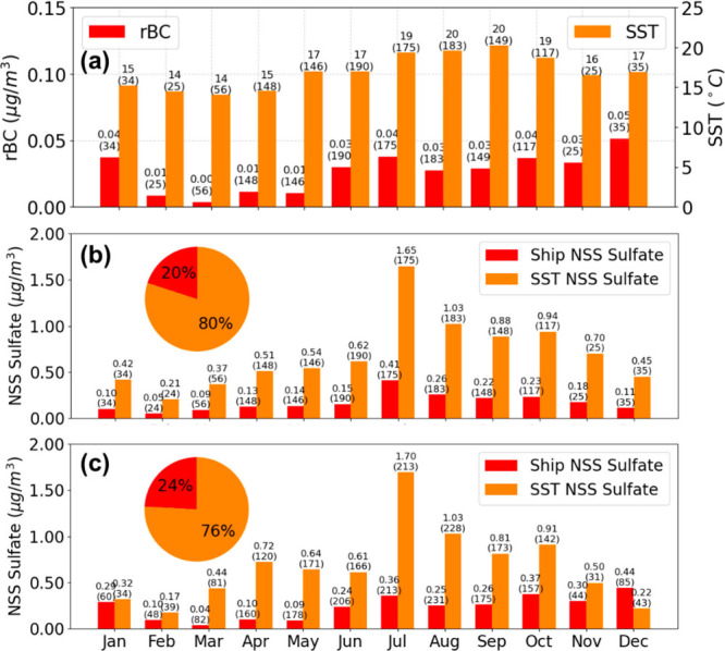
Aerosol nonsea-salt sulfate (NSS sulfate) forms in the atmosphere by secondary reactions of emissions from marine phytoplankton and shipping, with gas-phase as well as cloud and aerosol aqueous reactions controlling production. Twelve months of Atmospheric Radiation Measurements (ARM) during the Eastern Pacific Cloud Aerosol Precipitation Experiment (EPCAPE) at Scripps Pier in La Jolla, California, showed the highest NSS sulfate mass concentrations occurred for the northwesterly back-trajectories over 64% of the year, with an average of 0.90 μg/m³ that contributed 76% of annual NSS sulfate concentration. Multiple Linear Regression (MLR) and a refractory black carbon tracer method attributed 76-80% of the regionally emitted sulfur dioxide (SO₂) sources of submicron NSS sulfate to marine biogenic emissions and 20-24% to shipping emissions. MLR for oxidation processes explained 21% of the variability with Downwelling Shortwave Radiation (DSW) driving photochemical reactions to account for 34% of annual regional sulfate production, Upwind Cloud Vertical Fraction (UCVF) controlling cloud-associated oxidation to account for 29%, and relative humidity (RH) describing aerosol-phase oxidation to account for 36%. NSS sulfate was correlated moderately to UCVF during April-June and August but to RH in October-January. These findings show the apportionment of SO₂ emissions to biogenic and shipping sources and provide observational constraints for the mechanisms for sulfate production from SO₂ in the atmosphere.

Figure 1

Monthly boxplots of meteorological conditions during EPCAPE: (a) the average ambient air temperature (°C), (b) the downwelling shortwave radiation (DSW), (c) the average relative humidity (RH) (%), (d) the average upwind cloud vertical fraction (UCVF), and (e) the local cloud-mean liquid water content (LWC) (g/m³). (a) and (c) were retrieved and calculated from AOSMET at Scripps Pier, La Jolla, California. (e) was computed by utilizing the Minnis cloud products using VISST algorithm based on the trajectory starting at Scripps Pier and (b) and (d) were retrieved using the local measurements at Scripps Pier combining microwave radiometers and ARSCL retrievals.

Figure 2

Five identified transport clusters during EPCAPE with their PM1 mass fractions: 1) Coastal NW cluster (64%, Blue), 2) LA-LB cluster (18%, Red), 3) Southerly (6%, Green), 4) Easterly (9%, Orange), and 5) Marine Westerly (3%, Magenta). The cluster legend is shown on the top right and the cluster trajectory thickness represents the occurrence fraction of each cluster relative to the observed trajectories. The pie charts show each cluster’s PM1 aerosol composition as mass fractions with the average total PM1 mass concentrations (μg/m³) labeled in adjacent text. The PM1 composition legend (NR NSS sulfate (red), NR SS sulfate (yellow), NR organics (green), NR nitrate (blue), NR ammonium (orange), NR NSS chloride (light pink), rBC (black), sea salt (magenta) and dust (gray)) is shown on the top left.

Figure 3

(a) Monthly average fraction of transport cluster occurrence, accompanied by a pie chart illustrating the campaign occurrence fraction of each cluster relative to the observed trajectories. (b) PM1 aerosol mass concentrations, including NR NSS sulfate (red), NR SS sulfate (yellow), NR organics (green), NR nitrate (blue), NR ammonium (orange), NR NSS chloride (light pink), rBC (black), sea salt (magenta) and dust (gray), with a pie chart on the bottom right showing the annual averaged PM1 mass fraction.

Figure 4

Scatter plots and least-squares linear fits showing the relationship between the monthly median ship count per trajectory with (a) the monthly average rBC mass concentration (ng/m³) and (b) the monthly average NSS sulfate mass concentration (μg/m³). Data points are colored by month, and error bars are included. January and February 2024 were not shown as they are not available from AIS traffic data.

Figure 5

Frequency distribution of NSS sulfate/rBC ratios from the Coastal NW transport cluster, overlaid with NSS sulfate/rBC ratios reported from ship plumes in previous measurements off the California coast. The median and standard deviation of NSS sulfate/rBC ratios observed at Scripps Pier were 40 ± 80 during the Coastal NW cluster. The labels indicate ship plume characteristics, with corresponding number labels: (1) 0.62: Marine Diesel Oil (MDO) (0.07% sulfur content, speed 12 knots); (2) 0.8: MDO (0.1% sulfur content, speed 12 knots); (3) 1.4: Ultralow-sulfur diesel (ULSD) at 1600 rpm; (4) 1.7: MDO (0.1% sulfur content, speed 6.9 knots); (5) 6.2: MDO (0.1% sulfur content, speed 2.9 knots); (6) 6.4: Hydrogenation-Derived Renewable Diesel (HDRD) at 1600 rpm; (7) 11.3: HDRD at 700 rpm; (8) 13.2: Polluted marine atmosphere. References: (1) Lack et al., 2011; (2), (4), (5) Cappa et al., 2014; (3), (6), (7), (8) Price et al., 2017. The dashed black line at a ratio of 9.0 represents the baseline NSS sulfate/rBC ratio used in this study to estimate NSS sulfate from shipping emissions.

Figure 6

Scatter plots comparing the measured standardized regionally emitted NSS sulfate mass concentrations (μg/m³) against the predicted standardized NSS sulfate mass concentrations (μg/m³) from MLR models: (a) NSS sulfate (rBC, SST) and (b) NSS sulfate (DSW, UCVF, RH) using the data points from the CNW transport cluster.

Figure 7

(a) Monthly average rBC mass concentrations (μg/m³) (red, left y-axis) and SST (°C) (orange, right y-axis) per trajectory, with different scales on the y-axes. (b) Comparison of monthly average regionally emitted NSS sulfate mass concentrations (μg/m³) for source apportionment between NSS sulfate from ships (red) and SST (orange) using MLR analysis based on the CNW transport cluster. (c) Comparison of monthly average NSS sulfate from ships (red) and SST (orange) using the rBC-tracer method. Pie charts in (b) and (c) display the annual mass fractions of ship and SST NSS sulfate. Mean values are shown above each bar, with sample size in parentheses.

Figure 8

Monthly point-density scatter plots of NSS sulfate mass (μg/m³) vs Downwelling Shortwave Radiation. Linear regression lines are fitted where significant correlations are observed (r > 0.2 and p < 0.05), with the corresponding regression equation, Pearson correlation coefficient (r), and p-value indicated on the plots. The color darkness represents the relative point density.

Figure 9

Monthly point-density scatter plots of NSS sulfate mass (μg/m³) vs UCVF. Linear regression lines are fitted where significant correlations are observed (r > 0.2 and p < 0.05), with the corresponding regression equation, Pearson correlation coefficient (r), and p-value indicated on the plots. The color darkness represents the relative point density.

Figure 10

Monthly point-density scatter plots between NSS sulfate mass (μg/m³) and the measured RH (%) at the Scripps Pier. Linear regression lines are fitted where significant correlations are observed (r > 0.2 and p < 0.05), with the corresponding regression equation, Pearson correlation coefficient (r), and p-value indicated on the plots. The color darkness represents the relative point density.

Figure 11

Monthly secondary NSS sulfate mass concentrations per trajectory from source apportionment using MLR analysis comparing regionally emitted NSS sulfate mass contribution from downwelling shortwave radiation (DSW, yellow), upwind cloud vertical fraction (UCVF, blue) and relative humidity (RH, light blue) from the CNW transport cluster. The mean values are shown on top of each bar with and trajectory count in parentheses.

References

1. Seinfeld J.; Pandis S.. Atmospheric Chemistry and Physics: From Air Pollution to Climate Change, 3rd ed.; John Wiley & Sons, 2016.
1. Williams K. D.; Jones A.; Roberts D. L.; Senior C. A.; Woodage M. J. The Response of the Climate System to the Indirect Effects of Anthropogenic Sulfate Aerosol. Clim. Dyn. 2001, 17 (11), 845–856. 10.1007/s003820100150. - DOI
1. Kristjánsson J. E.; Iversen T.; Kirkevåg A.; Seland Ø.; Debernard J. Response of the Climate System to Aerosol Direct and Indirect Forcing: Role of Cloud Feedbacks. J. Geophys. Res. Atmospheres 2005, 110 (D24), 2005JD006299.10.1029/2005JD006299. - DOI
1. Sofiev M.; Winebrake J. J.; Johansson L.; Carr E. W.; Prank M.; Soares J.; Vira J.; Kouznetsov R.; Jalkanen J.-P.; Corbett J. J. Cleaner Fuels for Ships Provide Public Health Benefits with Climate Tradeoffs. Nat. Commun. 2018, 9 (1), 406.10.1038/s41467-017-02774-9. - DOI - PMC - PubMed
1. Fung K. M.; Heald C. L.; Kroll J. H.; Wang S.; Jo D. S.; Gettelman A.; Lu Z.; Liu X.; Zaveri R. A.; Apel E. C.; Blake D. R.; Jimenez J.-L.; Campuzano-Jost P.; Veres P. R.; Bates T. S.; Shilling J. E.; Zawadowicz M. Exploring Dimethyl Sulfide (DMS) Oxidation and Implications for Global Aerosol Radiative Forcing. Atmospheric Chem. Phys. 2022, 22 (2), 1549–1573. 10.5194/acp-22-1549-2022. - DOI
LinkOut - more resources