. 2025 Jun;9(6):1147-1161.
doi: 10.1038/s41562-025-02153-1. Epub 2025 Apr 17.

Differences in psychologists' cognitive traits are associated with scientific divides

Affiliations

Differences in psychologists' cognitive traits are associated with scientific divides

Justin Sulik et al. Nat Hum Behav. 2025 Jun.

Abstract

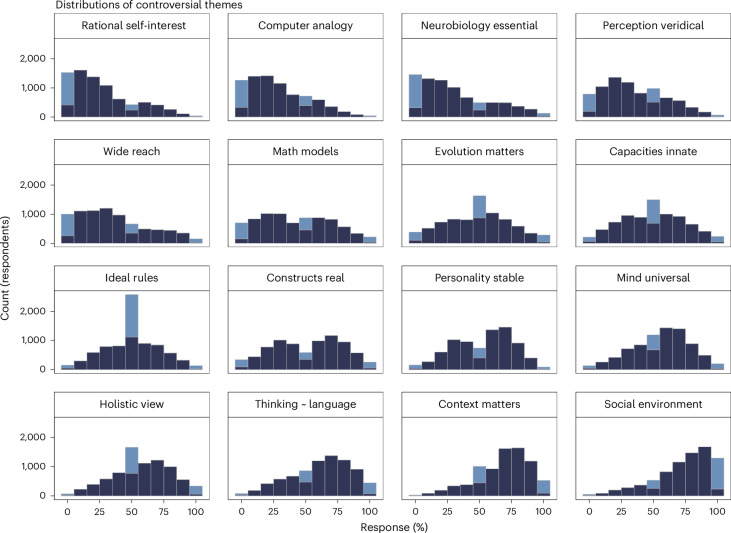
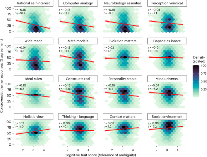
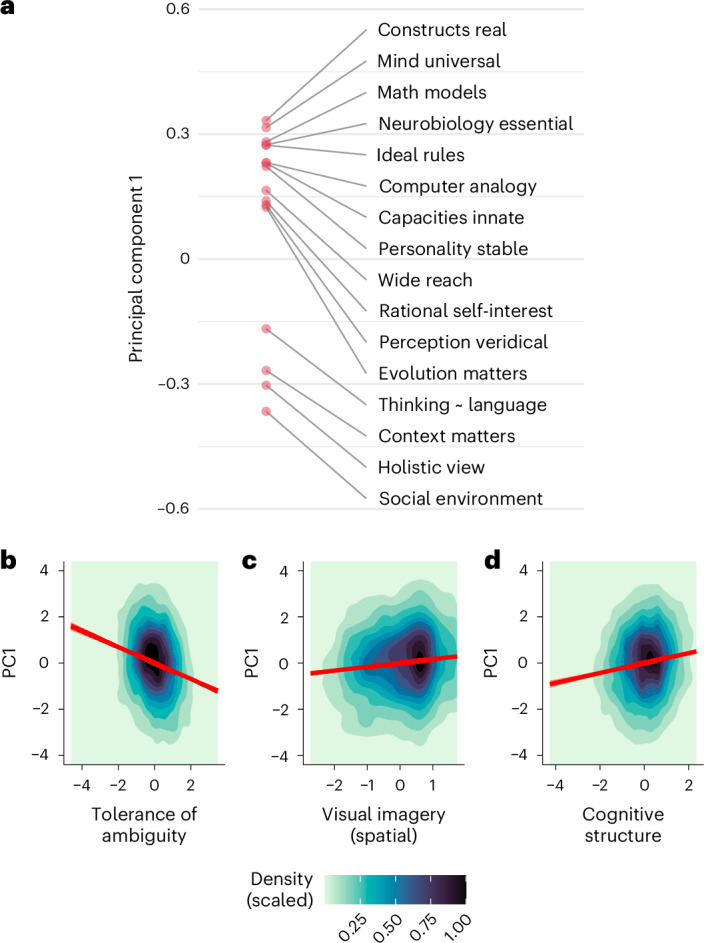
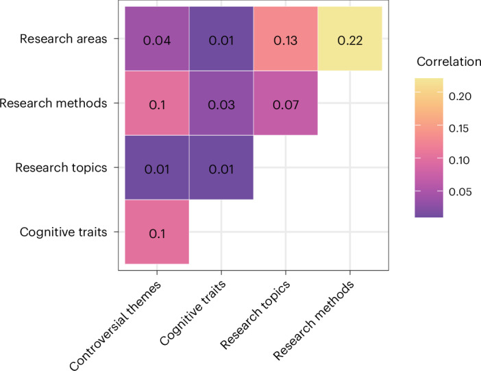
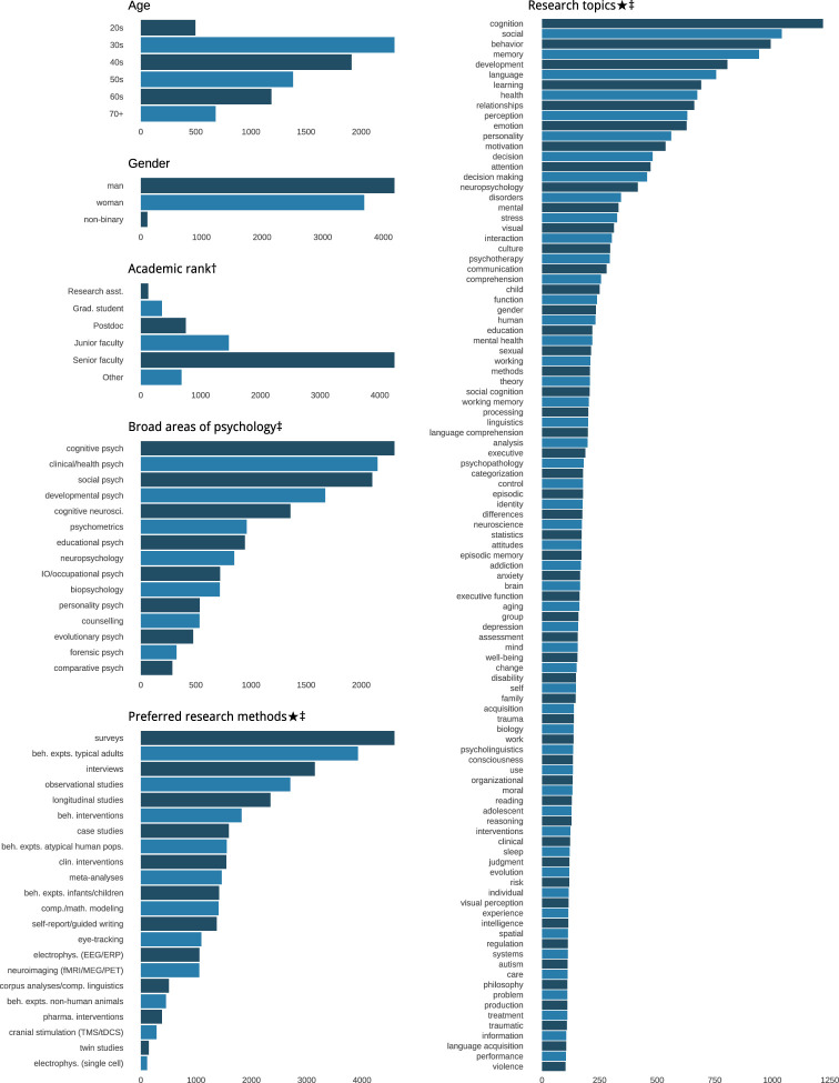
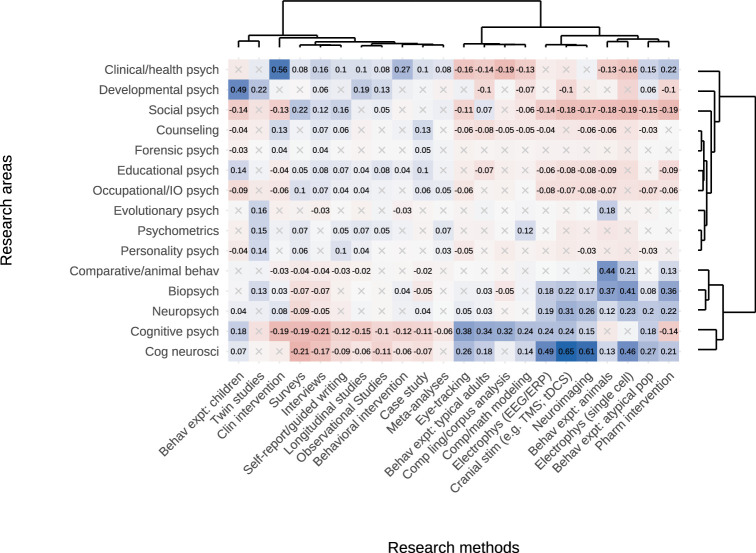
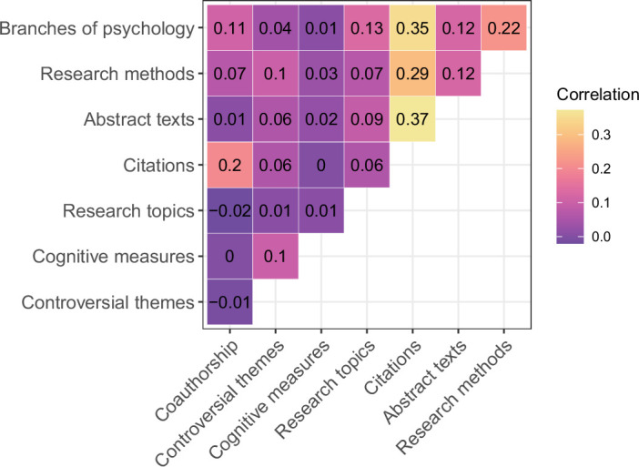
Scientific research is often characterized by schools of thought. We investigate whether these divisions are associated with differences in researchers' cognitive traits such as tolerance for ambiguity. These differences may guide researchers to prefer different problems, tackle identical problems in different ways, and even reach different conclusions when studying the same problems in the same way. We surveyed 7,973 researchers in psychological sciences and investigated links between what they research, their stances on open questions in the field, and their cognitive traits and dispositions. Our results show that researchers' stances on scientific questions are associated with what they research and with their cognitive traits. Further, these associations are detectable in their publication histories. These findings support the idea that divisions in scientific fields reflect differences in the researchers themselves, hinting that some divisions may be more difficult to bridge than suggested by a traditional view of data-driven scientific consensus.


Conflict of interest statement

Competing interests: J.E. has a commercial affiliation with Google, but Google had no role in the design and analysis of this study. The other authors declare no competing interests.

Figures

Fig. 1
Fig. 1. Histogram of responses to controversial themes.
Responses shown on a percentage scale where 100% represents complete agreement with the upper anchor label in Extended Data Table 1 and 0% represents complete agreement with the lower anchor label. Three distinctive response patterns are highlighted in lighter colour: extreme responses whereby participants moved the response slider all the way to 0 or 100%; and responses of exactly 50%, which necessitated moving the slider off the midpoint where it was initially, and then purposefully moving it back onto the midpoint (leaving it untouched on the midpoint would have prevented them from continuing to the next trial). Thus, for instance, the middle bin for theme ‘ideal rules’ contains some responses precisely at 50% in lighter blue and some responses near 50% in darker blue. Similarly, the left-most bin for theme ‘rational self-interests’ contains some responses exactly at 0% in light blue and some responses near 0% in dark blue. We highlight these distinct response strategies to emphasize the connection with regression models that quantify bimodality, extreme responses and midpoint spikes in Supplementary Table 1.
Fig. 2
Fig. 2. Controversial themes regressed on cognitive trait ‘tolerance of ambiguity’.
Illustrative plots of the linear relationships between each controversial theme and one of the cognitive traits: tolerance of ambiguity. Hexes show binned 2D density plots (with density scaled such that the peak density in each subpanel has a value of 1). Linear fits are shown in red (mean predictions with 99.9% CI ribbons). The correlation coefficient (Pearson’s r) corresponding to each fit is annotated in the top left of each panel, along with a t-value (for a full table of numeric results, see Supplementary Table 4). The OSF repository (https://osf.io/zyec9/) contains additional analyses, including non-parametric (Spearman’s r) models of the above, illustrating how these associations do not depend on an assumption of linearity. The OSF repository also contains similar plots for the other controversial themes, along with density plots for the binary variables such as research areas and methods.
Fig. 3
Fig. 3. Regression coefficients for controversial themes.
ad, Regression coefficients for controversial themes as a function of research areas, (b) research methods (b), cognitive traits (c) and gender (d). For tables of full numeric results, see Supplementary Tables 2–5. Cells marked ‘x’ are non-significant (with Bonferroni correction for multiple comparisons—the number of cells in each panel—yielding thresholds P < 0.000208 for a, P < 0.000142 for b and P < 0.000223 for c). All continuous variables are z-scored. Plot margins show hierarchical clusters (Ward’s method). d, In place of clusters for gender, given the low dimensionality of the space representing gender, two themes are shown where men gave lower scores than women and two with the reverse pattern (violin plots show full response distributions, with group means in red). For further distribution plots including non-binary participants, see the OSF repository at https://osf.io/zyec9/.
Fig. 4
Fig. 4. Three illustrative case studies, combining heterogeneous survey variables.
ac, Regression coefficients predicting three outcome variables. a, Whether researchers use computational/mathematical modelling in their work. b, Responses to controversial theme ‘neurobiology essential’. c, Responses to controversial theme ‘thinking ~ language’. Points show regression coefficients (with 95% CIs, reflecting sample sizes n = 7,865 for a; n = 7,973 for b and c). When the outcome variable is binary (a, ‘method’), the coefficients are expressed in logits. All continuous variables are z-scored, yielding standardized coefficients. Note that the x axes differ among panels to reflect the range of associations for three different outcomes.
Fig. 5
Fig. 5. Principal components representation of controversial themes, including associations with cognitive traits.
a, Themes projected onto the first principal component (PC1). bd, Individual differences in cognitive traits are associated with participants’ scores along the first principal component (PC1). Red lines show linear fits, overlaid on 2D density contour plots of the data (density scaled such that the peak density in each subpanel has a value of 1). For further details, see https://osf.io/nkbdr.
Fig. 6
Fig. 6. Exploratory factor analysis of controversial themes, including associations with cognitive traits.
a, Standardized loadings (lambdas) for a 5-factor exploratory factor analysis, representing how individual themes contribute to each latent factor. Cell colour indicates loading direction and strength (bluer, more positive; redder, more negative). Cell texts in white italic font merely highlight which latent factor each theme loads highest on. b, Standardized regression coefficients indicating how 6 cognitive traits predict latent factor scores (coefficient with 95% CIs, reflecting n = 7,973). Thus, the aforementioned latent factor 1 (‘essential’) is negatively associated with tolerance of ambiguity, positively associated with need for cognition and so on. For a numeric table of regression coefficients, see Supplementary Table 7.
Fig. 7
Fig. 7. Cosine similarities for the survey responses across abstract spaces representing each class of variable.
Correlations between cosine similarities across all pairs of participants, with vectors representing participants’ responses to each type of variable in the survey (controversial themes, cognitive traits, research topics, research methods, areas of psychology). For correlations including bibliometric models, see Extended Data Fig. 5.
Extended Data Fig. 1
Extended Data Fig. 1. Histograms of demographic and research variables.
† excluding respondents not in academia; ‡ respondents could choose more than one category; ⋆ plot truncated to show only counts > 100.
Extended Data Fig. 2
Extended Data Fig. 2. Distributions of research areas and methods projected onto a 2D UMAP representation of controversial themes.
Contour plots providing a high-level overview of how responses to controversial themes were distributed, projecting responses to all 16 themes onto a 2D space (UMAP parameters: number of nearest neighbors = 15; minimum distance = 0.1). Plot panels show distributions for (a) each research area; and (b) the most common research methods. These illustrate, for instance, how some research areas (for example, cognitive neuroscience, biopsychology) show greater concentration within this space than others (for example, social and developmental psychology are rather more dispersed). Shading represents density of the research area/methods responses associated with each participant in 2D space, not the controversial themes originally input into the UMAP algorithm. Density is scaled, such that the peak density in each sub-panel has a value of 1.
Extended Data Fig. 3
Extended Data Fig. 3. Distributions of cognitive trait variables.
Means ± 1SD (SD whiskers reflecting n=7973 except for Need for Cognition where n=6005).
Extended Data Fig. 4
Extended Data Fig. 4. Regression coefficients for research areas as a function of research methods.
Like Fig. 3, each cell here gives the regression coefficient for the simple model where individual research areas are regressed on individual research methods (though as the y-variable here is binary, unlike the controversial themes in Fig. 3, these are binomial regression coefficients expressed in logits). Cells marked with ‘x’ are non-significant (Bonferroni correction for multiple comparisons—the number of cells in the panel—yielding threshold p < .0001515). The margins of the plot show hierarchical clusters derived using Ward’s method. If the vectors of individual responses for research areas represent one high-dimensional space and the vectors of individual responses for research methods represent another high-dimensional space, then the correlation between all pairs of research-area vector cosine similarities and all pairs of research-methods cosine similarities is ρ = 0.22 (Figs. 5, 7), representing a conservative estimate for the overall association between these two types of response. For numeric results, see Appendix 2, Supplementary Table 6.
Extended Data Fig. 5
Extended Data Fig. 5. Cosine similarities for survey responses and bibliometric models across abstract spaces representing each class of variable.
Correlations between cosine similarities across all pairs of participants, with vectors either consisting of participants’ responses to each type of question in the survey (controversial themes, cognitive traits, research topics, research methods, areas of psychology) or extracted from three models of publication space: word embedding model of texts of abstracts and titles from an author’s published articles; network models representing the works cited in each article (thus representing the knowledge base assumed in the article); and patterns of co-authorship across those articles.
Extended Data Fig. 6
Extended Data Fig. 6. Regression coefficients predicting between-participant similarity in controversial themes and bibliometric models.
Regression coefficients for each set of predictors on outcomes variables (a) controversial themes; (b) semantic model of abstracts and titles; (c) citation model. Points indicate standardized coefficients with error bars reflecting 99%CIs (though in some cases these are too small to be seen clearly, relative to the size of the point representing the coefficient). For similarities within the survey data (panel a), CIs are based on n=6932 participants, yielding 24,022,846 unordered pairwise comparisons. For similarities across survey and bibliometric data (panels b, c), CIs are based on n=4829 participants, yielding 11,657,206 unordered pairwise comparisons.
Extended Data Fig. 7
Extended Data Fig. 7. Distributions of publication counts, split between survey respondents and those who were invited but did not respond.
Histograms showing the number of publications in journals classified as ‘psychology’ by WoS that we were able to index using the e-mail addresses to which invitations to participant were sent (using procedure identical to that described in Bibliometric models section of Materials). The top row shows the distribution of the survey respondents (median=6; mean=15.67). The bottom row shows the distribution of non-respondents, or e-mail addresses we emailed but did not get a survey response (median=3; mean=11.24). Note that the x-axis is broken after 210 for better visualization.
Extended Data Fig. 8
Extended Data Fig. 8. An overview of the inferred countries of email addresses to which we sent invitations, comparing those who responded with those who did not.
Our survey did not ask about participant’s geographic locations, and generic email domains such as ‘gmail.com’ do not license inferences about location. However, for university (or other institutional) email domains we are generally able to infer what countries those institutions are based in. We were able to do so for 6421 respondents so, even if this is not full coverage, it represents the bulk of the survey data. (a) A comparison of the log counts of those who responded to the survey and those who did not, with a linear fit (predicted log mean, with 95% CIs); (b) A comparison of the proportion represented by each country (as a percentage), either as a proportion of our survey respondents (blue) or as a proportion of invitation emails that did not receive a response (red); (c) A histogram of the difference between each country’s proportions from panel b, subtracting the proportion who did not respond from the proportion that did. For example, the largest value in the histogram is a difference of 8.36% percentage points representing the USA because 48.28% of our survey respondents had email domains in the US whereas 39.92% of emails that were invited but did not respond had the same. Given these indications that there is a good match in respondent vs non-respondent countries apart from the USA, which is somewhat over-represented, we believe our sampling strategy reached a wide range of participants (even if it is not a representative sample of the global academic psychology community).

Similar articles

References

    1. Campbell, D. T. in The Social Psychology of Science (eds Shadish, W. & Fuller, S.) Ch. 2 (Guilford Press, 1994).
    1. Koonon, E. V. & Wolf, Y. I. Is evolution Darwinian or/and Lamarckian? Biol. Direct4, 42 (2009). - PMC - PubMed
    1. Gergen, K. The social constructionist movement in modern psychology. Am Psychol.40, 266–275 (1985).
    1. Maines, D. The social construction of meaning. Contemp. Sociol.29, 577–584 (2000).
    1. Zerubavel, E. The five pillars of essentialism: reification and the social construction of an objective reality. Cult. Sociol.10, 69–76 (2016).

LinkOut - more resources