STForte: tissue context-specific encoding and consistency-aware spatial imputation for spatially resolved transcriptomics

Abstract

Encoding spatially resolved transcriptomics (SRT) data serves to identify the biological semantics of RNA expression within the tissue while preserving spatial characteristics. Depending on the analytical scenario, one may focus on different contextual structures of tissues. For instance, anatomical regions reveal consistent patterns by focusing on spatial homogeneity, while elucidating complex tumor micro-environments requires more expression heterogeneity. However, current spatial encoding methods lack consideration of the tissue context. Meanwhile, most developed SRT technologies are still limited in providing exact patterns of intact tissues due to limitations such as low resolution or missed measurements. Here, we propose STForte, a novel pairwise graph autoencoder-based approach with cross-reconstruction and adversarial distribution matching, to model the spatial homogeneity and expression heterogeneity of SRT data. STForte extracts interpretable latent encodings, enabling downstream analysis by accurately portraying various tissue contexts. Moreover, STForte allows spatial imputation using only spatial consistency to restore the biological patterns of unobserved locations or low-quality cells, thereby providing fine-grained views to enhance the SRT analysis. Extensive evaluations of datasets under different scenarios and SRT platforms demonstrate that STForte is a scalable and versatile tool for providing enhanced insights into spatial data analysis.

Keywords: deep learning; graph autoencoder; imputation; self-supervised learning; spatial transcriptomics.

Figure 1

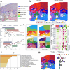
Schematic overview of our proposed approach. a, STForte processes SRT data to extract spatial KNN graph and expression feature matrix, identifying unmeasured or low-quality locations through automatic padding or user-defined procedures. b, The spatial graph contains consistency information while the feature attribute matrix captures expression heterogeneity, which are modeled and integrated using a pairwise autoencoder to learn latent encodings of feature attributes (ATTR) and spatial topology (TOPO), with adversarial distribution matching and feature propagation facilitating the modeling of association between these information types. c, The resulting encodings (ATTR, TOPO, and their concatenation COMB) can serve various analytical purposes. The illustration was created with BioRender.com.

Figure 2

a, H&E-stained image and annotation of the 10x Visium MOB data including a zoomed-in region. b, Spatial regions and UMAP visualization obtained from STForte (COMB encoding). c, Spatial regions and UMAP visualization under padding views obtained from STForte (TOPO encoding). d, Violin plots of gene expression levels of the selected five layer-specific marker genes. e, Visualization of the spatial expression levels of five layer-specific genes on the entire dataset (left) and the zoomed-in region (right). f, Spatial expression levels after STForte’s padding on the entire dataset (left) and the zoomed-in region (right). g, DAPI-stained image with manual annotation of the Stereo-seq MOB data. h, Spatial regions identified by different dimensional reduction methods, including STForte, STAGATE, and CA. i, UMAP visualizations obtained by different methods. j, Comparison of clustering metrics for different methods. k, Zoomed-in region of interest showing the results of low-quality spots processed by different methods.

Figure 3

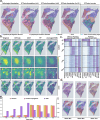
b, H&E-stained image with pathological annotations of the 10x Visium prostate adenocarcinoma. b, Spatial region identification using STForte ATTR encoding (left) and results from the padding scenario with STForte TOPO encoding (right). c, SC of STForte, CA, and STAGATE under the Leiden method at various resolutions. d, Spatial visualization shows the Leiden results from STAGATE and CA at their respective best SCs or when #Clust=11. e, Heatmap depicting the mean expression levels of genes associated with cancer, immune response, inflammation, and PGE synthesis across distinct spatial regions. The statistical significance of higher relative expression within each region was assessed using one-sided Wilcoxon rank-sum tests. The stars denote significance levels: *: P <0.05; **: P <0.001. f, Significant biological pathways associated with region C7 based on the differentially expressed genes. g, Spatial interaction between PTGES and PTGER4 genes based on STForte-identified regions and COMMOT analysis.

Figure 4

Example results of cancer edge identification with adjustment of and fine-grained gene expression padding. a, The manually combined cluster labels (ATTR encoding) under different values (left 1–4). Original Louvain clusters when (right 1). b, Visualization of the comparison between padded gene expression of STForte and other methods for cancer leading edge (LE) marker FABP5 and lymphocyte positive stroma (LPS) marker IGKC. c, Gene expression profiles of top highly variable genes in different tissue areas before and after gene padding. d, Clustering results of spatial domain padding (bottom) with randomly masked spots (top). e, Robustness of gene padding with randomly masked spots.

Figure 5

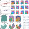
Investigations on the 10x Visium DLPFC dataset. a, Violin plot of spatial region identification performance across the 12 slices of the dataset using different approaches, quantified by the ARI and NMI metrics. The dashed lines represent the quartiles and median across 12 points. The asterisks denote significance levels: *: P 0.1; **: P 0.01; ns: P > 0.1. b, Spatial regions and performance metrics obtained by different approaches on slice No. 151673. c, Spatial (top) and UMAP visualization based on the COMB encoding (bottom) show the spot instances, including observed spots (Observed) and unmeasured intervals (Inferred), obtained by STForte’s padding strategy for slice No. 151673. d, Spatial visualizations of the propagated annotations of the padding scenario using spatial identification results (left) or manual annotation (right) based on TOPO encoding. e, UMAP visualization and trajectory analysis based on the COMB encoding for the propagated annotations. f, Trend plots display averaged expression levels of layer-specific marker genes based on the spatial region identified by STForte, ordered from WM to L1, with error bars showing standard deviations.

Figure 6

Analysis of Xenium mouse coronal brain data using STForte. a, Anatomical annotation of a coronal section of the mouse brain. Adapted from the Allen Brain Atlas. b, Spatial region identification based on STForte ATTR encoding on the Xenium mouse coronal brain dataset (top) and corresponding UMAP visualization (bottom). c, Spatial (top) and UMAP (bottom) visualizations of anatomical parcellation based on the summarized STForte results. d, Comparison of clustering performance metrics for different methods on this dataset. e, Visualization of the spatial regions identified by STForte in the Isocortex. f, Average expression levels of layer-specific marker genes in the outer cortical layers are shown with error bars representing the standard deviation. g, Hippocampal regions identified by STForte and the spatial expression patterns of relevant marker genes.

References

1. Cobb M. 60 years ago, Francis crick changed the logic of biology. PLoS Biol 2017;15:e2003243. 10.1371/journal.pbio.2003243 - DOI - PMC - PubMed
1. Marx V. Method of the year: Spatially resolved transcriptomics. Nat Methods 2021;18:9–14. 10.1038/s41592-020-01033-y - DOI - PubMed
1. Moses L, Pachter L. Museum of spatial transcriptomics. Nat Methods 2022;19:534–46. 10.1038/s41592-022-01409-2 - DOI - PubMed
1. Rao A, Barkley D, França GS. et al. Exploring tissue architecture using spatial transcriptomics. Nature 2021;596:211–20. 10.1038/s41586-021-03634-9 - DOI - PMC - PubMed
1. Zhu Q, Shah S, Dries R. et al. Identification of spatially associated subpopulations by combining scrnaseq and sequential fluorescence in situ hybridization data. Nat Biotechnol 2018;36:1183–90. 10.1038/nbt.4260 - DOI - PMC - PubMed