GC Content in Nuclear-Encoded Genes and Effective Number of Codons (ENC) Are Positively Correlated in AT-Rich Species and Negatively Correlated in GC-Rich Species

Abstract

Background/objectives: Codon usage bias affects gene expression and translation efficiency across species. The effective number of codons (ENC) and GC content influence codon preference, often displaying unimodal or bimodal distributions. This study investigates the correlation between ENC and GC rankings across species and how their relationship affects codon usage distributions.

Methods: I analyzed nuclear-encoded genes from 17 species representing six kingdoms: one bacteria (Escherichia coli), three fungi (Saccharomyces cerevisiae, Neurospora crassa, and Schizosaccharomyces pombe), one archaea (Methanococcus aeolicus), three protists (Rickettsia hoogstraalii, Dictyostelium discoideum, and Plasmodium falciparum),), three plants (Musa acuminata, Oryza sativa, and Arabidopsis thaliana), and six animals (Anopheles gambiae, Apis mellifera, Polistes canadensis, Mus musculus, Homo sapiens, and Takifugu rubripes). Genes in all 17 species were ranked by GC content and ENC, and correlations were assessed. I examined how adding or subtracting these rankings influenced their overall distribution in a new method that I call Two-Rank Order Normalization or TRON. The equation, TRON = SUM(ABS((GC rank₁:GC rank_N) - (ENC rank₁:ENC rank_N))/(N²/3), where (GC rank₁:GC rank_N) is a rank-order series of GC rank, (ENC rank₁:ENC rank_N) is a rank-order series ENC rank, sorted by the rank-order series GC rank. The denominator of TRON, N²/3, is the normalization factor because it is the expected value of the sum of the absolute value of GC rank-ENC rank for all genes if GC rank and ENC rank are not correlated.

Results: ENC and GC rankings are positively correlated (i.e., ENC increases as GC increases) in AT-rich species such as honeybees (R² = 0.60, slope = 0.78) and wasps (R² = 0.52, slope = 0.72) and negatively correlated (i.e., ENC decreases as GC increases) in GC-rich species such as humans (R² = 0.38, slope = -0.61) and rice (R² = 0.59, slope = -0.77). Second, the GC rank-ENC rank distributions change from unimodal to bimodal as GC content increases in the 17 species. Third, the GC rank+ENC rank distributions change from bimodal to unimodal as GC content increases in the 17 species. Fourth, the slopes of the correlations (GC versus ENC) in all 17 species are negatively correlated with TRON (R² = 0.98) (see Graphic Abstract).

Conclusions: The correlation between ENC rank and GC rank differs among species, shaping codon usage distributions in opposite ways depending on whether a species' nuclear-encoded genes are AT-rich or GC-rich. Understanding these patterns might provide insights into translation efficiency, epigenetics mediated by CpG DNA methylation, epitranscriptomics of RNA modifications, RNA secondary structures, evolutionary pressures, and potential applications in genetic engineering and biotechnology.

Keywords: CpG DNA methylation; GC content; bimodal distributions; codon bias; effective number of codons (ENC); epitranscriptomics; two-rank order normalization (TRON); unimodal distributions.

Figure 1

Bees (Apis mellifera), rice (Oryza sativa), and yeast (Saccharomyces cerevisiae) have different patterns of GC content and ENC ranks for nuclear-encoded genes. Figure 2d–f shows the three histograms separately for clarity. (a) Bees (blue), rice (red), and yeast (green) GC content (0.00 to 1.00) histograms of all nuclear-encoded genes (x-axis) are plotted against the number of genes with that range of GC content (y-axis). (b) Bees, rice, and yeast ENC level (20–61) histograms of all nuclear-encoded genes (x-axis) are plotted against the number of genes with that range of GC content (y-axis). The overlaps of the histograms are shown in different shades, as indicated.

Figure 2

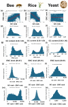
First column, bee (Apis mellifera), second column, rice (Oryza sativa), and third column, yeast (Saccharomyces cerevisiae) correlations between GC content and ENC level for nuclear-encoded genes. (a–c) Correlations between ENC ranks (y-axis) and GC ranks (x-axis) for bees, rice, and yeast. ENC rank was determined by sorting all columns based on ENC levels (20–61) and then numbering the rows 1-N, where N is the number of genes in that species. GC rank was determined by sorting all columns based on GC levels (0.00–1.00) and then numbering the rows 1-N. When GC levels are sorted and all columns are selected, the original ranks of the ENC levels are maintained. Correlations between ENC levels and GC levels by selecting the ENC ranked column and making a scatter plot (shown in blue bars). Trend lines were made by right-clicking (control clicking) a point on the graph and selecting TRENDLINES (red arrows). Under TRENDLINES, select boxes for set intercept (=INTERCEPT(GCrank:ENCrank)), display equation on chart, and display R-squared value on chart (shown). Notice that bees have a positive correlation, rice has a negative correlation, and yeast has no correlation between ENC rank and GC rank (red arrows). (d–f) GC histograms for bees, rice, and yeast. The GC contents (0–1.00) for all nuclear-encoded genes are on the x-axis and the number of genes with that range of GC values is on the y-axis. Histograms were made by selecting the GC column and selecting histogram chart under the INSERT tab. Notice that bees and rice have bimodal distributions of GC content and Yeast has a unimodal distribution. (g–i) ENC histograms for bees, rice, and yeast. The ENC levels (20–61) for all nuclear-encoded genes are on the x-axis and the number of genes with that range of ENC levels are on the y-axis. Notice that bees and rice have bimodal distributions of ENC and Yeast has a unimodal distribution. (j–l) GC rank minus ENC rank histograms for bees, rice, and yeast. Notice that GC rank minus ENC rank (GC-ENC) is unimodal in bees and bimodal in rice. (m–o) GC rank plus ENC rank histograms for bees, rice, and yeast. Notice that GC+ENC is bimodal in bees and unimodal in rice. This is the opposite of the pattern in (j–l).

Figure 3

GC and ENC analyses with negative correlations between GC rank and ENC rank: Mosquito (Anopheles gambiae), pufferfish (Takifugu rubripes), human (Homo sapiens), bread mold (Neurospora crass), banana (Musa acuminata), and mouse (Mus musculus). (a) Mosquito GC rank (y-axis) versus ENC rank (x-axis) shows a negative correlation. X-axis is 1 to 12,402 for the rank order of the 12,402 nuclear encoded mosquito genes based on GC content (0.00 to 1.00). Y-axis is 1 t0 12,402 for the rank order of genes based on GC levels, sorted on ENC rank (see Figure 2). (b) Mosquito histogram of GC content (0 to 1.00) versus the number of genes (N) that fall within the indicated range of GC content. (c) Mosquito histogram of ENC levels (0 to 1.00) versus the number of genes (N) that fall within the indicated range of ENC levels. (d) Mosquito histogram of GC rank—ENC rank versus the number of genes (N) that fall within the indicated range of GC rank—ENC rank. The x-axis is −12,402 to +12,402. (e) Mosquito histogram of GC rank + ENC rank versus the number of genes (N) that fall within the indicated range of GC rank + ENC rank. The x-axis is 1 to 2 × 1204, which is two times the number of nuclear-encoded genes in mosquitoes. (f–j) Pufferfish analyses (as described in (a–e)) for the 22,104 nuclear-encoded genes in this species. (k–o) Human analyses (as described in (a–e)) for the 19,708 nuclear-encoded genes in this species. (p–t) Bread mold analyses (as described in (a–e)) for the 9728 nuclear-encoded genes in this species. (u–y) Banana analyses (as described in (a–e)) for the 30,700 nuclear-encoded genes in this species. (z–dd) Mouse analyses (as described in (a–e)) for the 22,405 nuclear-encoded genes in this species.

Figure 4

GC and ENC analyses of species with positive correlations between GC rank and ENC rank: wasp (Polistes canadensis), rickettsia (Rickettsia hoogstraalii), slime mold (Dictyostelium discoideum), arabidopsis (Arabidopsis thaliana), and plasmodium (Plasmodium falciparum). (a–e) Wasp analyses (as described in Figure 4) for the 9854 nuclear-encoded genes in this species. (f–j) Rickettsia analyses (as described in Figure 4) for the 1663 nuclear-encoded genes in this species. (k–o) Slime mold analyses (as described in Figure 4) for the 13,078 nuclear-encoded genes in this species. (p–u) Arabidopsis analyses (as described in Figure 4) for the 10,160 nuclear-encoded genes in this species. (v–y) Plasmodium analyses (as described in Figure 4) for the 5321 nuclear-encoded genes in this species.

Figure 5

GC and ENC analyses of species with little or no correlations between GC rank and ENC rank: E. coli (Escherichia coli), pombe (Schizosaccharomyces cerevisiae), and methanobacteria (Methanococcus aeolicus). (a–e) E. coli analyses (as described in Figure 4) for the 10,276 nuclear-encoded genes in this species. (f–j) Pombe analyses (as described in Figure 4) for the 5110 nuclear-encoded genes in this species. (k–o) Methobacteria analyses (as described in Figure 4) for the 1485 nuclear-encoded genes in this species.

Figure 6

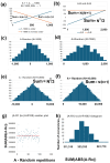
Combinatorial effects of adding or subtracting GC and ENC ranks. (a) Line A (1, 2, …, 1000) (red) and Line B (1000, 999, …, 1) are plotted. Column A on Excel™ has the numbers for Line A and column B has the numbers for Line B. (b) Line A minus Line B (A−B) (blue) and Line A+B (red) are plotted. A−B was made by selecting column A (rows 1–1000) and subtracting column B (rows 1–1000) and placing the results in column C. A+B was made by selecting column 1 and adding column 2 and placing the results in column D. (c) A histogram of Line A minus a randomization of Line A (Random) is plotted (A-Random). Random was generated on Excel™ with the RANDARRAY function, i.e., =SORTBY(A₁:A₁₀₀₀,RANDARRAY(1000)). The results were placed in column E. The histogram was made by selecting column E (rows 1–1000) and selecting the histogram chart under the INSERT tab. (d) A histogram of Line A plus a randomization of Line A (R) is plotted (A+Random). The results of A+Random was inserted into column F. (e) A histogram of Line A’ (1, 2, …, 10,000) (column G) minus a randomization of A’ (column H) and placed in column I (A’-Random’). The steps in C were repeated using numbers 1–10,000 for line A’ and randomization of numbers 1–10,000 for Random’. The area was determined by the equation (SUM(ABS(I₁:I_10,000). ABS (absolute value) was used in this equation because half of the numbers are negative. The area can also be approximated as N²/3, where N is the number of rows, in this case there are 10,000 rows (see methods). (f) A histogram of Line A’ plus Random’ and placed in column J (A’+Random’). The area was determined by the equation (SUM(J₁:J_10,000)) = N(N + 1)/2. (g) A scatter plot of 100 repetitions of SUM(ABS(A₁:A₁₀₀₀) − (R₁:R₁₀₀₀)), where R is a randomization of the numbers between 1 and 1000 using the equation SORTBY(A₁:A₁₀₀₀,RANDARRAY(1000). The red line shows the average = 333,023 +/− 7360, which is equivalent to N²/3 +/− 2%. (h) A histogram of the results in g, where the x-axis is SUM(ABS(A₁:A₁₀₀₀) − (R₁:R₁₀₀₀)) and the y-axis is the number of times that range of number occurred in 100 repetitions.

Figure 7

Correlations between GC content, ENC, and the number of nuclear-encoded genes. Data for all graphs is from Table 1. (a) Plot of TRON score (y-axis) versus slope (GC rank vs. ENC rank) (x-axis) for all 17 species. Species with negative slopes between GC ranks and ENC ranks are on the left and species with positive slopes are on the right. The trendline and R-squared value is shown. TRON score is SUM(ABS((GC₁:GC_N) − (ENC₁:ENC_N))/(N²/3). (b) Plot of R-squared correlation (y-axis) versus slope (GC rank vs ENC rank) (x-axis) for all 17 species. Species with negative slopes between GC ranks and ENC ranks are on the left and species with positive slopes are on the right. The polynomial trendline and R-squared value is shown. (c) GC content at peak 1 (y-axis) versus number of nuclear-encoded genes (x-axis) for all 17 species. The trendline and R-squared value is shown. (d) GC content at peak 2 (y-axis) versus number of nuclear-encoded genes (x-axis) for all 17 species. The trendline and R-squared value is shown. (e) ENC level at peak 1 (y-axis) versus GC content at peak 1 (x-axis) for all 17 species. The trendline and R-squared value is shown. (f) ENC level at peak 2 (y-axis) versus GC content at peak 1 (x-axis) for all 17 species. The trendline and R-squared value is shown.

References

1. Plotkin J.B., Kudla G. Synonymous but not the same: The causes and consequences of codon bias. Nat. Rev. Genet. 2011;12:32–42. doi: 10.1038/nrg2899. - DOI - PMC - PubMed
1. Wright F. The ’effective number of codons’ used in a gene. Gene. 1990;87:23–29. doi: 10.1016/0378-1119(90)90491-9. - DOI - PubMed
1. Liu X. A more accurate relationship between ’effective number of codons’ and GC3s under assumptions of no selection. Comput. Biol. Chem. 2013;42:35–39. doi: 10.1016/j.compbiolchem.2012.11.003. - DOI - PubMed
1. Sharp P.M., Li W.H. The codon Adaptation Index—A measure of directional synonymous codon usage bias, and its potential applications. Nucleic Acids Res. 1987;15:1281–1295. doi: 10.1093/nar/15.3.1281. - DOI - PMC - PubMed
1. Puigbò P., Bravo I.G., Garcia-Vallvé S. E-CAI: A novel server to estimate an expected value of Codon Adaptation Index (eCAI) BMC Bioinform. 2008;9:65. doi: 10.1186/1471-2105-9-65. - DOI - PMC - PubMed
LinkOut - more resources