Learning via mechanosensitivity and activity in cytoskeletal networks

Abstract

In this work we show how a network inspired by a coarse-grained description of actomyosin cytoskeleton can learn - in a contrastive learning framework - from environmental perturbations if it is endowed with mechanosensitive proteins and motors. Our work is a proof of principle for how force-sensitive proteins and molecular motors can form the basis of a general strategy to learn in biological systems. Our work identifies a minimal biologically plausible learning mechanism and also explores its implications for commonly occuring phenomenolgy such as adaptation and homeostatis.

FIG. 1.

Physical learning via structural remodeling in a model inspired by the cytoskeleton: (A) Our model is a disordered spring network of nodes connected by edges. The source and target edges are indicated in color. The learning mechanism involves supervised driving at the target edge. (B) Schematic representation of the molecular mechanism of learning showing the dynamic coupling between the network elasticity and agents mimicking molecular motors and mechanosensitive proteins that can bind/unbind from each edge. (C) Schematic showing how driving at the target edge creates local strain and enables an update of the learning degree of freedom (rest length) at any arbitrary edge of the network, via mechanosensation and active force generation. (D) Learning dynamics in one edge of the network. The change in the learning degree of freedom (rest length) at the edge in response to active forces generated by motor dynamics. The dashed line indicates where the active force reaches the threshold active force value $f^a=g_c$ above which rest length changes according to the learning rule.

FIG. 2.

Learning strain response in cytoskeletal networks by changing rest lengths. (A) Time evolution of training error over many cycles of exposure to desired behavior. (inset) The network at the initial unstrained state. The source and target edges are denoted by “S” and “T” respectively. (B) Trained network reflecting the magnitude of changes in the rest length $\left(\left|\text{Δ}{L}_0\right|\right)$ of the edges given by the edge thickness. The colors indicate if the rest length increased (red) or decreased (blue) with respect to the original rest length values after training. (C) The strain at the target edge on the application of the source strain on the trained network. The untrained response at the target edge is shown in a red dashed line which is far from the desired target strain (gray dashed line) (D) Training error vs training time at different values of activity given by the contractility parameter $\xi$. Here the rescaled parameter values are $k=1$, $\xi =0.5$, $\beta =0.1$, $k_u=0.5$, ${\lambda }_{\max }=0.5$ and $\alpha =1$.

FIG. 3.

Learning strain response in cytoskeletal networks by changing stiffness. (A) Time evolution of training error over many cycles of exposure to desired behavior. (B) The trained network topology and edge stiffness change $|\text{Δ}k|$ which is proportional to line width. The source and target edges are denoted by “S” and “T” respectively. (C) The strain at the target edge on the application of the source strain in the trained network. The untrained response at the target edge is shown in a red dashed line, which is far from the desired target strain (gray dashed line). (D) Learning with non-linear protein dynamics and non-linear elasticity. Training error vs training time shows that increasing the strength of nonlinearity in both the protein dynamics $\left({\beta }_2,{\beta }_3\ne 0\right)$ and network elasticity $\left(k_2,k_3\ne 0\right)$ leads to lower training errors. The numbers in the legend indicate these parameter values. We consider a simple case of the same values for the unitless nonlinear coefficients ${\beta }_2={\beta }_3=0.1$, $k_2=-0.1$ & $k_3=0.1$ with other parameters same as Fig. 2 except ${\lambda }_{max}=0.2$ and $\xi =0.2$. For panels (A-C) the rescaled parameter values are $\xi =5$, $\beta =0.1$, $k_u=0.5$, ${\lambda }_{\max }=10$ and $\alpha ={10}^3$.

FIG. 4.

Classification of environmental signals in cytoskeletal networks. (A) Schematic showing a cell in an environment with a strain gradient. (B) Environmental mechanical signal as the positive and negative gradient of strain. The strain pattern input is imposed on source edges (green) and two target edges are chosen to encode the two classes “+” (purple) and “ − ” (orange). (C) Training error vs training time for both positive and negative strain gradients as inputs. (D) Classification accuracy increases as the training progresses. The network learns to classify faster with higher activity (given by contractility parameter $\xi$). Here ${\tau }_f/{\tau }_s=1/10$, ${ϵ}_T^{\ast (+)}=-{ϵ}_T^{\ast (-)}=0.25$, ${\mathcal{E}}_{tol}=0.025$ and the rescaled parameter values are same as used in Fig. 2 except $\alpha =10$.

FIG. 5.

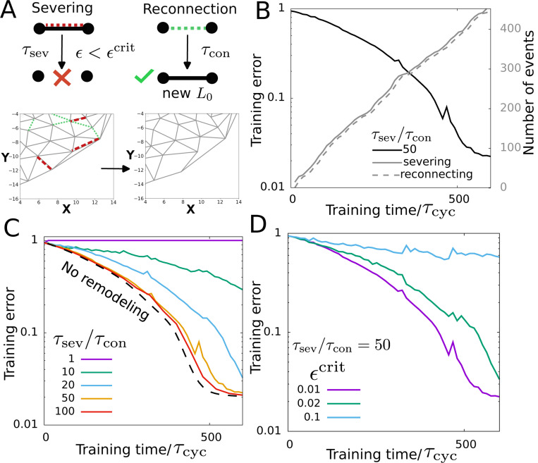
Learning in the presence of network turnover. (A) The schematic on the top shows edge severing and reconnection processes. The bottom part shows an example of network remodeling. Green and red dashed lines mark the bonds to get created and severed respectively. (B) Training in the presence of network remodeling. Training error decreases over time. The solid and the dashed gray lines show the number of severing and reconnection events as the training progresses. (C) Training error as a function of the training time at various severing timescales $\left({\tau }_{\text{sev}}\right)$. The dashed line shows training without remodeling. (D) Training error with training time at different critical strain values ${ϵ}^{\text{crit}}.{\tau }_{\text{sev}}/{\tau }_{\text{con}}=50$. The parameter values used here are the same as Fig. 2 except ${ϵ}^{\text{crit}}=0.01$, ${\tau }_{\text{con}}=10{\tau }_{\text{cyc}}$.

FIG. 6.

Activity dependent recovery from loss of learning. (A) Training error for different activity values (given by the contractility parameter $\xi$) for ${\tau }_{\text{sev}}/{\tau }_{\text{con}}=9$. (B) A phase diagram in activity and rescaled severing timescale. The arrow indicates the direction of the faster turnover of network edges. The parameter values used here are the same as Fig. 2. Additionally ${ϵ}^{\text{crit}}=0.01$, ${\tau }_{\text{con}}=10{\tau }_{\text{cyc}}$.

FIG. 7.

Self-organized learning via actomyosin pulsation. (A) Schematic showing self-organized pulse driving the target edge instead of the supervisor. (B) Target strain with training time for driving by pulses of constant amplitude $A=A_0$. (C) Target strain with training time for driving by pulses with target edge length $\text{(}L\text{)}$ dependent feedback $A=a_{0}L$. Here ${\tau }_f/{\tau }_s=1/4$ and the rescaled parameter values are $\beta =0.1$, $k_u=0.4$, $\xi =1$ and $\alpha =1$.

FIG. 8.

Interplay between motor dynamics, activity and mechanosensitivity enables self-organized learning. (A) Example of trained networks in three different cases corresponding to the points highlighted by broken circles in the phase diagram. (B) Phase diagram showing phases of No learning (white), Conserved geometry learning (gray shaded) and altered geometry learning (yellow shaded) at different values of activity parameter $\xi$ and motor turnover rate $k_u$. (C) Phase diagram showing phases of No learning (white), Conserved geometry learning (gray shaded) and altered geometry learning (yellow shaded) at different values of activity parameter $\xi$ and a measure of mechanosensitivity ${\beta }_1$ (same as $\beta$ in rescaled units). The phases are determined from visualization of trained networks and the boundaries are lines drawn as guides to the eyes. Here ${\tau }_f/{\tau }_s=1/4$ and the rescaled parameter values are $\beta =0.1$ (in panel B), $k_u=0.5$ (in panel C), and $\alpha =10$.

FIG. 9.

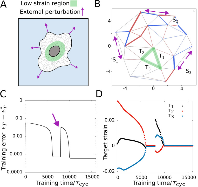
Adaptation via learning. (A) Schematic showing desired low-strain region in the cell in the presence of external mechanical perturbations. (B) The trained network shows the external forces acting on the network (magenta arrows) and the low-strain region in green. (C) Training error reduces obtaining the desired target strain value ${ϵ}_T^{\ast }=0$ for all target edges. (D) Target strain values with training time at three target edges. The ${\tau }_{\text{cyc}}$ and rescaled parameter values are the same as Fig. 2 except $\alpha =10$.

References

-
- Gunst Susan J, Tang Dale D, and Saez Anabelle Opazo. Cytoskeletal remodeling of the airway smooth muscle cell: a mechanism for adaptation to mechanical forces in the lung. Respiratory physiology & neurobiology, 137(2–3):151–168, 2003. - PubMed
- Guillot Charlène and Lecuit Thomas. Mechanics of epithelial tissue homeostasis and morphogenesis. Science, 340(6137):1185–1189, 2013. - PubMed
- Arzash Sadjad, Tah Indrajit, Liu Andrea J, and Manning M Lisa. Rigidity of epithelial tissues as a double optimization problem. Physical Review Research, 7(1):013157, 2025.
- Tah Indrajit, Haertter Daniel, Crawford Janice M, Kiehart Daniel P, Schmidt Christoph F, and Liu Andrea J. A minimal vertex model explains how the amnioserosa avoids fluidization during drosophila dorsal closure. Proceedings of the National Academy of Sciences, 122(1):e2322732121, 2025. - PMC - PubMed
Publication types
Grants and funding
LinkOut - more resources
Full Text Sources