Metaplasticity and continual learning: mechanisms subserving brain computer interface proficiency

Abstract

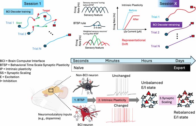
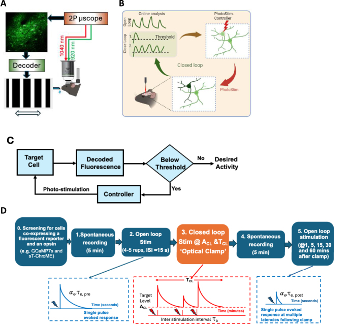
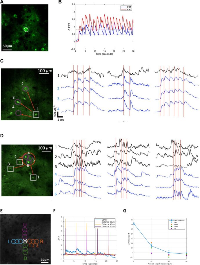
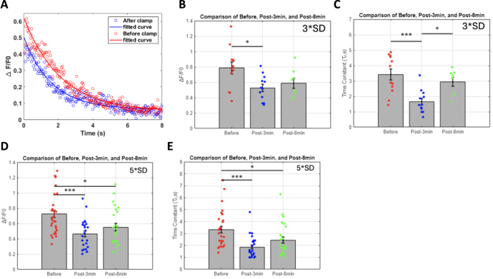
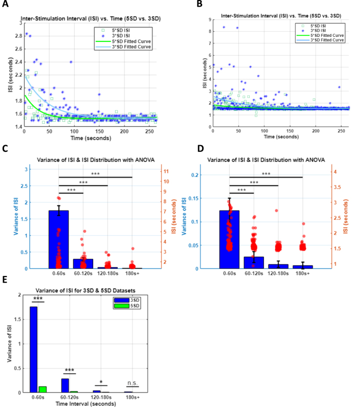
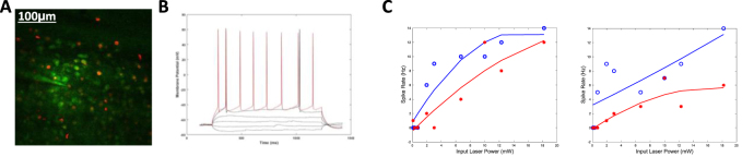
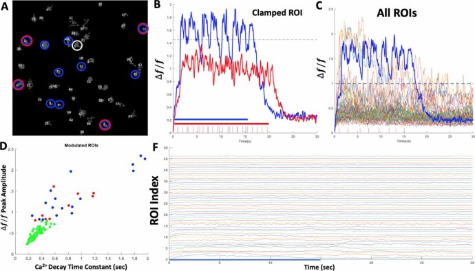
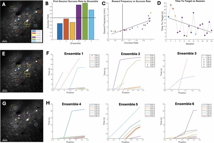
Objective.Brain computer interfaces (BCIs) require substantial cognitive flexibility to optimize control performance. Remarkably, learning this control is rapid, suggesting it might be mediated by neuroplasticity mechanisms operating on very short time scales. Here, we propose a meta plasticity model of BCI learning and skill consolidation at the single cell and population levels comprised of three elements: (a) behavioral time scale synaptic plasticity (BTSP), (b) intrinsic plasticity (IP) and (c) synaptic scaling (SS) operating at time scales from seconds to minutes to hours and days. Notably, the model is able to explainrepresentational drift-a frequent and widespread phenomenon that adversely affects BCI control and continued use.Approach.We developed an all-optical approach to characterize IP, BTSP and SS with single cell resolution in awake mice using fluorescent two photon (2P) GCaMP7s imaging and optogenetic stimulation of the soma targeted ChRmine_Kv2.1. We further trained mice on a one-dimensional BCI control task and systematically characterized within session (seconds to minutes) learning as well as across sessions (days and weeks) with different neural ensembles.Main results.On the time scale of seconds, substantial BTSP could be induced and was followed by significant IP over minutes. Over the time scale of days and weeks, these changes could predict BCI control proficiency, suggesting that BTSP and IP might be complemented by SS to stabilize and consolidate BCI control.Significance.Our results provide early experimental support for a meta plasticity model of continual BCI learning and skill consolidation. The model predictions may be used to design and calibrate neural decoders with complete autonomy while considering the temporal and spatial scales of plasticity mechanisms. With the power of modern-day machine learning and artificial Intelligence, fully autonomous neural decoding and adaptation in BCIs might be achieved with minimal to no human intervention.

Keywords: BCI; calcium imaging; cognitive control; learning; optogenetics; synaptic plasticity.

Figure 1.

Meta plasticity model for BCI learning and skill consolidation featuring interaction between three elements: behavioral time scale synaptic plasticity (BTSP), intrinsic plasticity (IP) and synaptic scaling (SS) taking place over a multitude of time scales. During the first BCI training session (top left), rewarded neural activity patterns result in an increase in their frequency through BTSP (bottom left). The sensory feedback inputs arriving at different times along the cursor trajectory would then be potentiated if they are most relevant to the agent’s rewarded behavior (green arrows) and would be depressed if they lead to reward prediction error (red arrows). Through neuromodulatory influence and repeated activation, changes in intrinsic excitability result and may persist over longer periods, depending on the frequency of training (top and bottom middle). This shifted homeostatic state leads to an unbalanced excitation/inhibition (E/I) state that could also affect non-BCI neurons within the local circuits (bottom right). The balance is eventually restored through synaptic scaling over much slower time scales. The restoration of this balance might not re-instate the original excitability state of each individual neuron but may result in a new ‘attractor’ state of the ensemble representing the learned experience. These changes could explain the representational drift typically observed over similar time scales that adversely affects BCI performance and requires repeated BCI decoder calibration in subsequent sessions (top right).

Figure 2.

(A). Schematic illustration of an all optical exogenous BCI experiment. Rewarded neural ensemble activity instantly decoded and used as a control signal drive a ‘neural cursor’ on the screen in the form of orientation gratings. (B). Endogenous BCI experiment uses the instantly decoded fluorescence (e.g. Ca²⁺imaged througha two-photon (2P)microscope at920 nm) to directly photo stimulate the same (or different) neuron(s) co-expressing an opsin in closed loop at a non-overlapping spectral wavelength (1040 nm). (D). Protocol for characterizing BTSP and IP over a full experimental session. The open loop photo stimulation is used to measure the effects of performing the closed loop approach at disjoint intervals. In this open loop step, each cell is photo stimulated with a single depolarizing pulse (4–5 repetitions, separated by 15 s for a total duration of ∼1 min) and the evoked fluorescence Ca²⁺ traces are averaged to obtain a baseline for a proxy of the global dendritic plateau potential before the closed loop step (optical clamp). The open loop step is repeated at multiple time points following cessation of the clamp. The parameters $\alpha$_e and τ_e are used to characterize the changes in the plateau potential’s amplitude and time constant observed in each case. (C). Endogenous BCI operation using an optical clamp: the decoded fluorescence is compared to a user specified threshold target activity level A_CL, either in the same cell or in other cells within the field of view (FOV). If the activity drops below the target level, photo stimulation is delivered to depolarize the cell keep its activity above that level and the cycle continues for a user specified interval T_CL.

Figure 3.

(A). Example FOV with a single neuron (white circle) co-expressing ChRmine_Kv2.1 and GCaMP7s targeted for closed loop photo stimulation based on the protocol in figure 2(B). (B). Sample Ca²⁺ traces of the clamped neuron in A at two different target activity levels: mean + 3*standard deviation (SD) and mean + 5*SD for 30 s. Ca²⁺ imaging was acquired at 30 Hz over an FOV of ∼250 × 250 μm using a resonant galvo scanning system at 920 nm and photo stimulated neurons via two-photon excitation at 1040 nm. The spatial light modulator (SLM, Meadowlark Optics, CO) generated a single photo stimulation spot, which was scanned in a spiral fashion for 50 ms (5 spirals) per pulse. (C). Examples of single and (D). population optical clamping. Grey square and traces are trigger neurons. Blue circles and traces are stimulated target neurons that are ‘yoked’ together. Red lines indicate stimulation trigger times conditioned on activity decoded from the trigger neurons. (E). A ∼250 × 250 μm FOV demonstrating the stimulation spots used to verify stimulation off target effects and 4 directions around the target cell body. (F). Example Ca²⁺ traces from ‘off center’ color coded locations at 3 different spatial distances. (G). Ca²⁺ fluorescence decay profile at photo stimulation spots ‘off center’ according to (E) and (F).

Figure 4.

Characterization of somatic Ca²⁺ response to open loop stimulation (A). Example average change in Ca²⁺ impulse response to single pulse open loop stimulation, a proxy of the plateau potential, before and after optical clamp at 5*SD of baseline fluorescence for 200 s. (B). Changes in peak Ca²⁺ amplitude $\alpha$_e following clamp at 3*SD target level (before vs post-3 min: *p = 0.011 035) that partially rebounded at 8 min (before vs post-8 min: p = 0.065 906; post-3 min vs post-8 min: p = 0.473 26) (n = 3 cells, N = 3 mice). (C). Change in Ca²⁺ decay time constant τ_e following clamp at 3*SD target level (before vs post-3 min: ***p = 0.000 517 85; before vs post-8 min: p = 0.312 63; post-3 min vs post-8 min: *p = 0.003 2513) (n = 3 cells, N = 3 mice). (D). Changes in peak Ca²⁺ amplitude $\alpha$_e following clamp at 5*SD target level (before vs post-3 min: ***p = 0.000 101 67; before vs post-8 min: *p = 0.015 294; post-3 min vs post-8 min: p = 0.1656). (n = 7 cells, N = 3 mice). (E). Change in Ca²⁺ decay time constant τ_e following clamp at 5*SD target level (before vs post-3 min: ***p = 4.9042 × 10⁻⁰⁵; before vs post-8 min: *p = 0.024 711; post-3 min vs post-8 min: p = 0.076 848). (n = 7 cells, N = 3 mice).

Figure 5.

Characterization of somatic Ca²⁺ response to closed loop stimulation (A). Example inter stimulation interval (ISI) and exponential curve fitting associated with clamping one example cell at 3*SD and 5*SD. (B). Same as in A but for n = 5 cells across N = 4 mice. (C). ISI and its variance during clamp broken down by 60 s intervals for target activity level 3*SD. Optical parameters used are power = 10 mW; 161 pulses per 266 s (or 36 pulses min⁻¹). 0–60 s, 60–120 s: ***p = 9.50 × 10⁻⁰⁶; 0–60 s, 120–180 s: ***p = 6.68 × 10⁻¹⁰; 0–60 s-180+: ***p = 1.25 × 10⁻¹²; 60–120 s, 120–180 s: p = 0.385; 60-120 ,180+: p = 0.132; 120–180 s,180+: p = 0.964. (D). Same as C but with target 5*SD resulting in 168 pulses per 266 s (or 38 pulses min⁻¹). [0–60 s, 60–120 s]: ***p = 2.13 × 10⁻⁰⁹; [0–60 s, 120–180 s]: ***p = 2.36 × 10⁻¹⁵;[0–60 s-180+]: ***p = 4.37 × 10⁻¹³; [60–120 s, 120–180 s]: p = 0.266; [60-120 ,180+]: p = 0.350; [120-180 s,180+]: p = 0.99. (E). Comparison of ISI and its variance across two different levels across all cells in all mice (two-sample t-test: time interval 0–60 s: ***p = 0.000 03; 60–120 s: ***p = 0.000 74; 120–180s: *p = 0.014 64; 180s+: p = 0.642 71).

Figure 6.

Characterization of changes in intrinsic excitability before and after optical clamp (A). representative field of view for two photon-guided whole-cell recording in current clamp mode to characterize the cell’s f–I response. (B). Sample whole cell membrane voltage recordings to two depolarizing current levels (5 $\mu$ A black, 10 $\mu$ A red) and multiple non-depolarizing current levels. (C). Power-frequency characteristics before and after clamp (at 5*SD target level for 200 s) for two example cells. Blue open circles and red asterisks represent input laser power (proxy for the current injected) to spike rate before and after clamp, respectively.

Figure 7.

Influence of clamped neuron on adjacent neurons within the same FOVA. (A) Example FOV containing 46 well isolated ROIs in mouse V1. ROI#5 (circled in white) was selected for optical clamping at two target levels shown in B. ROIs circled in red are cell bodies showing significant increase in Ca²⁺ fluorescence intensity in response to target level (3*SD) in B. ROIs circled in blue are cell bodies showing significant increase in Ca²⁺ fluorescence intensity in response to clamp level (5*SD). (B) Activity of the clamped ROI#5 in A and photo stimulation pulse trains used for each target level (red 3*SD, blue 5*SD). (C) Raw Ca²⁺ fluorescence of all ROIs in the FOV during clamp interval for target 5*SD for comparison. ROIs showing significant modulation synchronized with the clamped ROI (n = 17/46 cells, 5*SD target, **p = 0.0011) correspond to blue circled ROIs in A. (D) Ca²⁺ peak fluorescence versus decay time constant for all 46 ROIs in the FOV for target level 5*SD in C. Each dot represents the average of Ca²⁺ peak fluorescence and event decay time constant locked to each photo stimulation pulse during the clamp. Green dots are ROIs that were not significantly modulated within the clamp period (n = 29; p = 0.152). (F) Raw Ca²⁺ fluorescence for all 46 ROIs in A at target 5*SD. Significantly modulated ROIs are plotted consecutively to demonstrate the difference between the activated and non-activated ROIs shown in C following cessation of the clamp at 15 s.

Figure 8.

(A). FOV where six different ensembles of 4 neurons each were used to train the animal on the BCI task over 6 different sessions. Some ensembles overlapped whereas others did not. (B). Success rate in the first session for each of the ensembles in (A). Dashed line indicate a threshold of 60% success that was used to categorize the ensembles into either a ‘weak/slow learner’ (E1–E3) or a’strong/rapid learner” ensemble (E4–E6). (C). Average time to target in each session (color coded by ensemble) demonstrating continuous decrease over sessions for ensemble E4. (D). Time to target (TT) over sessions for ensemble E4 and for session 1 of the other 5 ensembles. Strong learner ensembles E4–E6 exhibited a TT = 6.21 ± 6.1 s over 20 sessions compared to TT = 17.8 ± 20.2 s for the weak learner ensembles E1–E3. (E). Same FOV as A but highlighting only the neurons selected for ensembles E1–E3 using the same color code in A. (F). Cursor path from initial start position to target position in the first 7 trials of the first session for ensembles E1–E3. Dashed lines indicate incomplete trial, whereas x indicates a failed trial (timeout). (G). Same FOV as A but highlighting only the neurons selected for ensembles E1–E3 using the same color code in A. (H). Cursor path from initial start position to target position in the first 7 trials of the first session for ensembles E4–E6.

Figure 9.

(A). Average firing rate of BCI neurons during BCI control in the same ensemble (E4) comparing an early session versus a later session (2 weeks apart). Each dot represents the average firing rate over a 50 s interval within ∼10 min of behavioral trials. Success rate in both sessions was 90% and 98%, respectively. (B). Baseline firing rate comparison for the same ensemble in (A) outside of BCI behavioral sessions. Each dot represents the average firing rate over a 50 s interval within ∼8 min. (C). Baseline firing rate of non-BCI neurons in the same sessions as A. Each dot represents the average firing rate over a 50 s interval within ∼8 min (p = 0.013; 0.000 85; 3.77 × 10⁻⁰⁵; 0.756; 0.598 for neurons N1–N5 respectively, two-sided t-test).

References

1. Hochberg L R, Serruya M D, Friehs G M, Mukand J A, Saleh M, Caplan A H, Branner A, Chen D, Penn R D, Donoghue J P. Neuronal ensemble control of prosthetic devices by a human with tetraplegia. Nature. 2006;442:164–71. doi: 10.1038/nature04970. - DOI - PubMed
1. Collinger J L, et al. High-performance neuroprosthetic control by an individual with tetraplegia. Lancet. 2013;381:557–64. doi: 10.1016/S0140-6736(12)61816-9. - DOI - PMC - PubMed
1. Wodlinger B, Downey J E, Tyler-Kabara E C, Schwartz A B, Boninger M L, Collinger J L. Ten-dimensional anthropomorphic arm control in a human brain-machine interface: difficulties, solutions, and limitations. J. Neural Eng. 2015;12:016011. doi: 10.1088/1741-2560/12/1/016011. - DOI - PubMed
1. Collinger J L, et al. Collaborative approach in the development of high-performance brain-computer interfaces for a neuroprosthetic arm: translation from animal models to human control. Clin. Transl. Sci. 2014;7:52–59. doi: 10.1111/cts.12086. - DOI - PMC - PubMed
1. Guan C, Aflalo T, Kadlec K, Gámez de Leon J, Rosario E R, Bari A, Pouratian N, Andersen R A. Decoding and geometry of ten finger movements in human posterior parietal cortex and motor cortex. J. Neural Eng. 2023;20:036020. doi: 10.1088/1741-2552/acd3b1. - DOI - PMC - PubMed
LinkOut - more resources