A visual-omics foundation model to bridge histopathology image with transcriptomics

Abstract

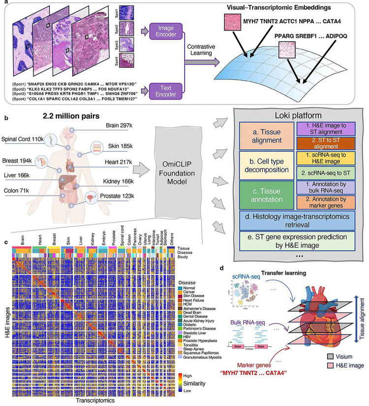
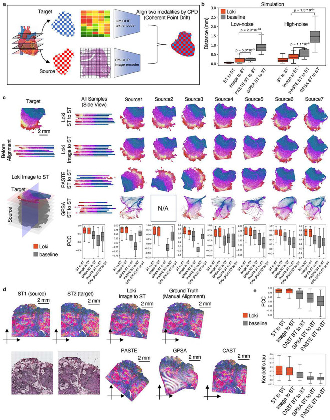
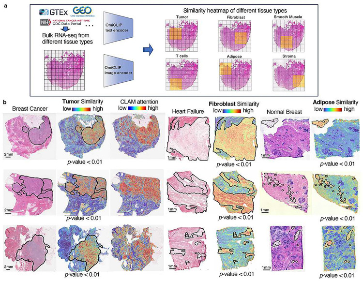
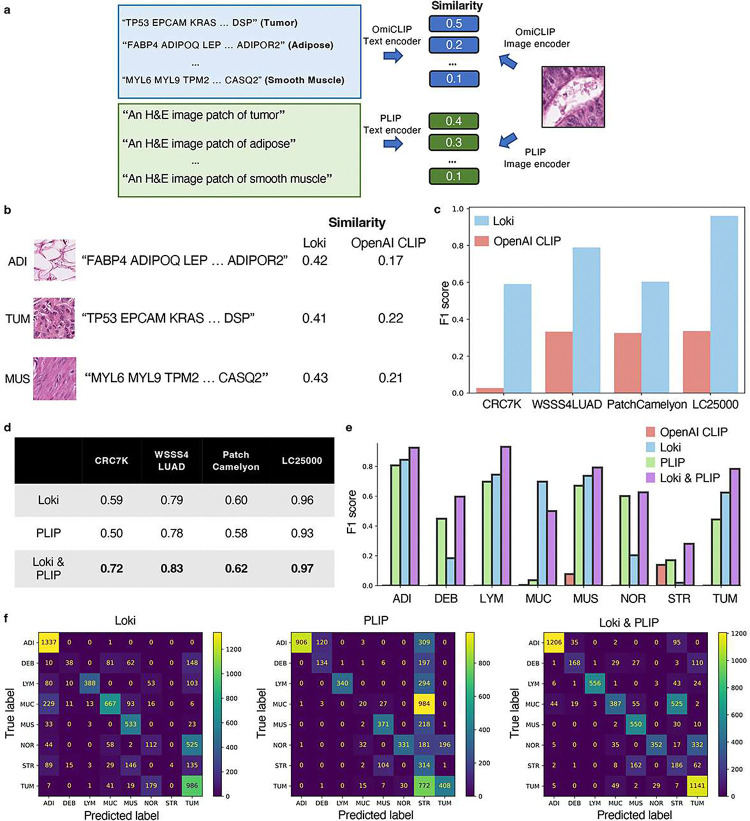
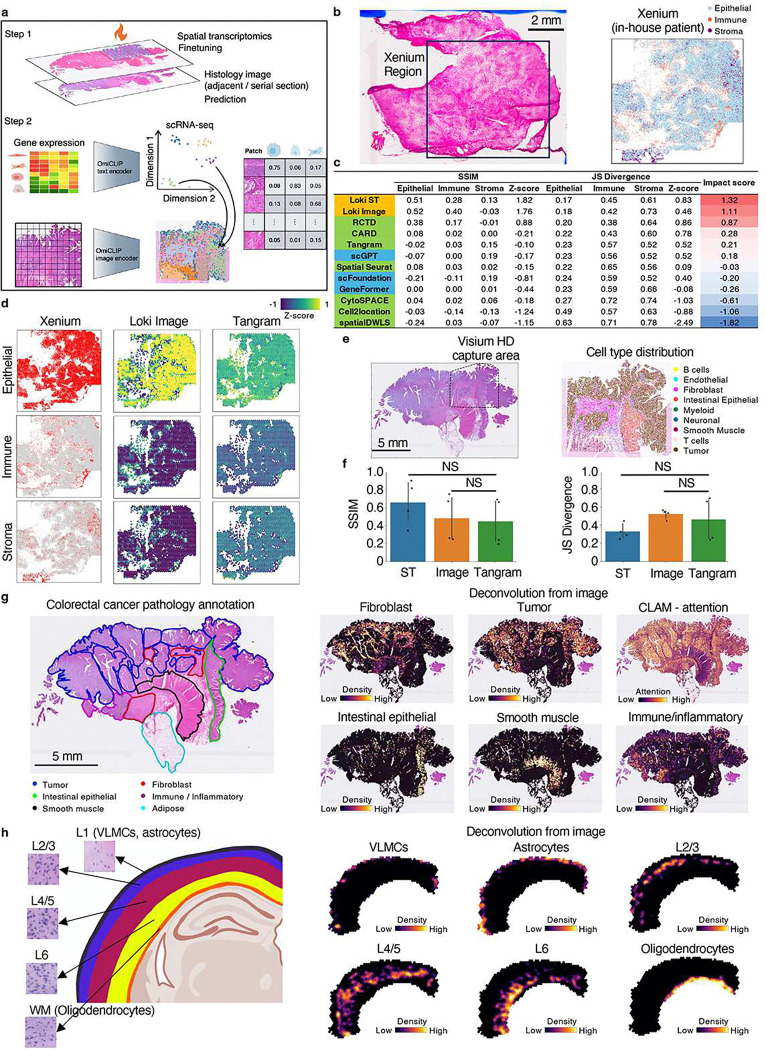
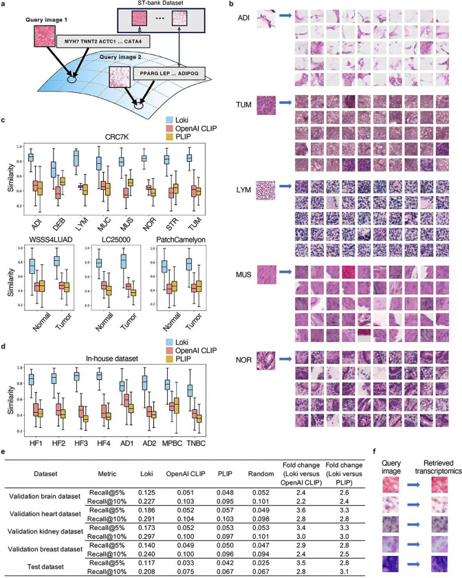
Artificial intelligence has revolutionized computational biology. Recent developments in omics technologies, including single-cell RNA sequencing (scRNA-seq) and spatial transcriptomics (ST), provide detailed genomic data alongside tissue histology. However, current computational models focus on either omics or image analysis, lacking their integration. To address this, we developed OmiCLIP, a visual-omics foundation model linking hematoxylin and eosin (H&E) images and transcriptomics using tissue patches from Visium data. We transformed transcriptomic data into "sentences" by concatenating top-expressed gene symbols from each patch. We curated a dataset of 2.2 million paired tissue images and transcriptomic data across 32 organs to train OmiCLIP integrating histology and transcriptomics. Building on OmiCLIP, our Loki platform offers five key functions: tissue alignment, annotation via bulk RNA-seq or marker genes, cell type decomposition, image-transcriptomics retrieval, and ST gene expression prediction from H&E images. Compared with 22 state-of-the-art models on 5 simulations, 19 public, and 4 in-house experimental datasets, Loki demonstrated consistent accuracy and robustness.

Figure 1. Overview of the study.

a, The work ow of pre-training the OmiCLIP model with paired image–image-transcriptomics dataset via contrastive learning. b, The work ow of Loki platform using OmiCLIP foundation model as an engine. Left diagram illustrates the size of the training data in different organs. Right diagram lists the existing modules of the Loki platform, including tissue alignment, cell type decomposition, tissue annotation, ST gene expression prediction, and histology image–transcriptomics retrieval. Created in BioRender. c, The heatmap represents image embeddings and transcriptomic embeddings similarity across various organs and disease conditions. The color of the heatmap reflects the OmiCLIP’s embedding similarities, with red indicating high similarity and blue with low similarity. d, Schematic illustration of Loki platform with transfer learning for 3D tissue analysis. Created in BioRender.

Figure 2. Tissue alignment.

a, Schematic illustration of tissue alignment using ST and histology image with Loki Align. Created in BioRender. b, Performance comparison of tissue alignment on 100 low-noise and 100 high-noise simulated datasets, represented by the distance between ground truth and aligned simulated sample using Loki (ST to ST and Image-to-ST) and baseline methods PASTE (ST-to-ST) and GPSA (ST-to-ST), respectively. P-values were calculated using a one-sided Wilcoxon test. c, Alignment results on 8 adjacent normal human small intestine samples using Loki (ST-to-ST and Image-to-ST) and baseline methods PASTE (ST-to-ST), GPSA (ST-to-ST) and CPD method (ST-to-ST), respectively. We colored the samples using the top three PCA components of OmiCLIP transcriptomic embeddings, mapped to red, green, and blue color channels, respectively. For visualization, we stack the 8 samples together along the perpendicular axis before and after different alignment methods respectively, and visualize from the side view. The source2 that has no spatial variable gene selected by GPSA to run it, is marked as N/A. Boxplots show the comparison of tissue alignment performances on these 7 source samples respectively and combined, represented by the PCC (and Kendall’s tau coefficient in Extended Fig. 4a) of highly variable gene expression between target and source sample after alignment at the same location, using Loki and baseline methods (PASTE, GPSA and CPD method using PCA embeddings as input) respectively. In the box plots, the middle line represents the median, the box boundaries indicate the interquartile range, and the whiskers extend to data points within 1.5× the interquartile range. d, Tissue alignment of 2 adjacent human ovarian carcinosarcoma samples using Loki (ST-to-ST and Image-to-ST) and baseline methods PASTE (ST-to-ST), GPSA (ST-to-ST) and CAST (ST-to-ST), respectively. We colored the samples as described in b. e, Alignment performance comparison using PCC and Kendall’s tau coefficient of the highly expressed gene expression between target sample and source sample at aligned locations, using Loki (ST-to-ST and Image-to-ST) and baseline methods PASTE (ST-to-ST), GPSA (ST-to-ST) and CAST (ST-to-ST), respectively. In the box plots, the middle line represents the median, the box boundaries indicate the interquartile range, and the whiskers extend to data points within 1.5× the interquartile range, n=147.

Figure 3. Tissue annotation using bulk RNA-seq data.

a, Schematic illustration of tissue annotation using H&E image and reference bulk RNA-seq data from different sources, with OmiCLIP paired image and transcriptomic embeddings. b, Histology WSIs of breast cancer, heart failure, and normal breast samples. The major tumor regions, broblast cell enriched regions, and adipose regions are annotated by pathology experts in black lines. Heatmap shows the similarity of WSIs to the corresponding reference bulk RNA-seq of tumor, broblast, and adipose, respectively. The color of the heatmap reflects the similarities between WSIs and reference bulk RNA-seq data, with red indicating high similarity and blue with low similarity. CLAM attention heatmaps were generated using CLAM with default parameters.

Figure 4. Tissue annotation using marker genes.

a, Schematic illustration of tissue annotation using H&E image and reference marker genes. The annotation result is decided by choosing the candidate texts with the highest similarity score to the input image query. For Loki, we used the text content of marker gene symbols of each tissue type. For PLIP model, we used the text content of natural language description of each tissue type. b, Examples of similarity scores of images and texts calculated by Loki and OpenAI CLIP model, respectively. c,Comparison of zero-shot performances, represented by weighted F1 scores, across four datasets using Loki and OpenAI CLIP model, respectively. Number of test samples for each dataset are CRC7K (n = 6,333); WSSS4LUAD (n = 10,091); LC25000 (n = 15,000); and PatchCamelyon (n = 32,768). d, Comparison of zero-shot performances, represented by weighted F1 scores, across four datasets using Loki, PLIP model, and incorporating Loki and PLIP models by average similarity (shown in panel a, Methods), respectively. e, Comparison of zero-shot performances, represented by weighted F1 scores of each tissue type in the CRC7K dataset using OpenAI CLIP model, Loki, PLIP model, and incorporating Loki and PLIP models, respectively. f, Confusion matrix of the CRC7K dataset using Loki (left), PLIP model (middle), and incorporating Loki and PLIP models (right), respectively. The ground truth labels are presented in rows and the predicted labels are presented in columns. Adipose tissue abbreviated as ADI, normal colon mucosa abbreviated as NOR, colorectal carcinoma epithelium abbreviated as TUM, lymphocytes abbreviated as LYM, mucus abbreviated as MUC, debris abbreviated as DEB, smooth muscle abbreviated as MUS, and cancer-associated stroma abbreviated as STR.

Figure 5. Cell type decomposition.

a, Schematic illustration of tissue alignment using ST, reference scRNA-seq data, and histology image with OmiCLIP paired transcriptomic and image embeddings after finetuning. b, H&E image of our in-house triple-negative breast cancer (TNBC) patient sample, characterized by Xenium into three major cell types: cancer epithelial, immune, and stromal cells. c, Performance comparison of 12 decomposition methods using JS divergence, SSIM, and impact scores. Z-scores of JS divergence (or SSIM) across methods was calculated based on the average JS divergence (or SSIM) among cell types. The impact score of each method is the average of the z-score of JS divergence and SSIM (Methods). The green color indicates decomposition tools. The blue color indicates the performance of replacing OmiCLIP embeddings with other transcriptomic foundation models’ embeddings. d, Cell type decomposition results on three major cell types of the TNBC sample using the image by Loki and using ST by Tangram, with Xenium data as ground truth. The color of the heatmap reflects the z-score, calculated by the probability distribution of each cell type. e, H&E image of the human colorectal cancer sample and cell type distribution within the Visium HD capture area. f, Bar plot shows the accuracy of decomposition on four major cell types by Loki using ST or image, and by Tangram using ST. Error bar is standard deviation with center measured by mean. For both JS divergence and SSIM, adjusted p-value > 0.1 using a two-sided Wilcoxon test. g, Whole-slide (20mm×13mm) human colorectal cancer cell type decomposition. Different tissue regions are annotated by the pathologist as ground truth. Heatmap shows the cell type distribution of broblast, tumor, intestinal epithelial, smooth muscle, and immune/inflammatory, with color reflecting the density of each cell type. CLAM attention heatmaps were generated using CLAM with default parameters. h, Cell type decomposition results on the brain sample. Left: brain anatomical references with zoom-in H&E image patches of L1 (VLMCs, astrocytes), L2/3, L4/5, L6, and WM (oligodendrocytes), respectively. Created in BioRender. Right: heatmap shows the cell type distribution of VLMCs, astrocytes, L2/3, L4/5, L6, and oligodendrocytes, with color reflecting the distribution of each cell type.

Figure 6. Image-to-transcriptomics retrieval.

a, Schematic illustration of Image-to-transcriptomics retrieval on the ST-bank dataset. b, Example image-to-transcriptomics retrieval results. For each example image from adipose, colorectal adenocarcinoma epithelium, lymphocytes, smooth muscle, and normal colon mucosa, the retrieved top 50 most similar transcriptomics are shown by the paired image from the ST-bank dataset. c, Image-to-transcriptomics retrieval similarity scores across the four validation datasets: CRC7K, WSSS4LUAD, LC25000, and PatchCamelyon using Loki, OpenAI CLIP, and PLIP respectively. In the box plots, the middle line represents the median, the box boundaries indicate the interquartile range, and the whiskers extend to data points within 1.5× the interquartile range. d,Image-to-transcriptomics retrieval similarity scores across the 8 in-house patient tissues: heart failure (HF), Alzheimer’s disease (AD), metaplastic breast cancer (MPBC), and triple-negative breast cancer (TNBC), using Loki, OpenAI CLIP, and PLIP respectively. In the box plots, the middle line represents the median, the box boundaries indicate the interquartile range, and the whiskers extend to data points within 1.5× the interquartile range. e, Image-to-transcriptomics retrieval evaluation across four validation datasets and one test dataset using Loki, OpenAI CLIP, and PLIP, respectively, with random baseline. The top-K quantile most similar transcriptomics were retrieved. We report Recall@K for K ∈ {5%, 10%} (Methods). f, Example image-to-transcriptomics retrieval results. The retrieved transcriptomics are shown by the paired image.

References

1. Hegde N., et al. Similar image search for histopathology: SMILY. NPJ digital medicine 2, 56 (2019). - PMC - PubMed
1. Chen C., et al. Fast and scalable search of whole-slide images via self-supervised deep learning. Nature biomedical engineering 6, 1420–1434 (2022). - PMC - PubMed
1. Huang Z., et al. Artificial intelligence reveals features associated with breast cancer neoadjuvant chemotherapy responses from multi-stain histopathologic images. NPJ Precision Oncology 7, 14 (2023). - PMC - PubMed
1. Lu M.Y., et al. AI-based pathology predicts origins for cancers of unknown primary. Nature 594, 106–110 (2021). - PubMed
1. Zhu L., et al. An accurate prediction of the origin for bone metastatic cancer using deep learning on digital pathological images. EBioMedicine 87(2023). - PMC - PubMed
Publication types
LinkOut - more resources