Longitudinal profiling of low-abundance strains in microbiomes with ChronoStrain

Abstract

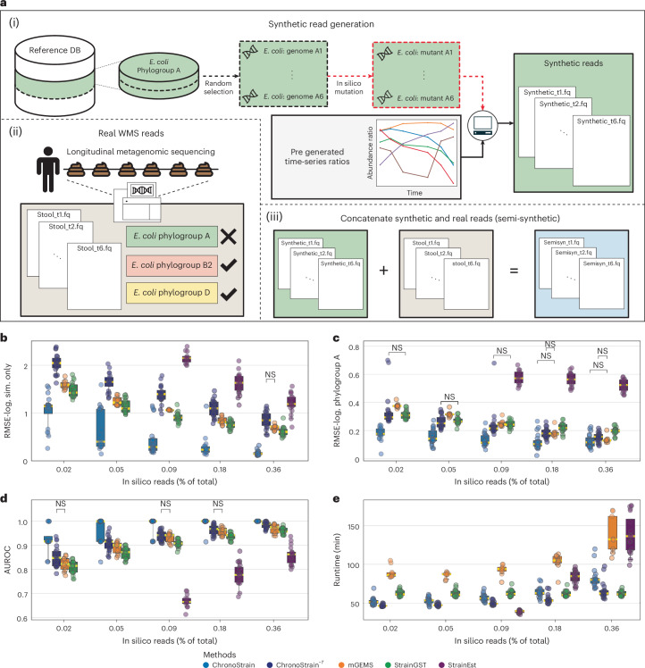
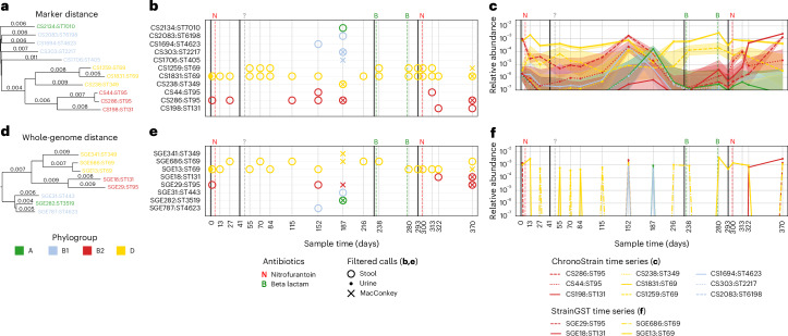
The ability to detect and quantify microbiota over time from shotgun metagenomic data has a plethora of clinical, basic science and public health applications. Given these applications, and the observation that pathogens and other taxa of interest can reside at low relative abundance, there is a critical need for algorithms that accurately profile low-abundance microbial taxa with strain-level resolution. Here we present ChronoStrain: a sequence quality- and time-aware Bayesian model for profiling strains in longitudinal samples. ChronoStrain explicitly models the presence or absence of each strain and produces a probability distribution over abundance trajectories for each strain. Using synthetic and semi-synthetic data, we demonstrate how ChronoStrain outperforms existing methods in abundance estimation and presence/absence prediction. Applying ChronoStrain to two human microbiome datasets demonstrated its improved interpretability for profiling Escherichia coli strain blooms in longitudinal faecal samples from adult women with recurring urinary tract infections, and its improved accuracy for detecting Enterococcus faecalis strains in infant faecal samples. Compared with state-of-the-art methods, ChronoStrain's ability to detect low-abundance taxa is particularly stark.

Fig. 1. Overview of ChronoStrain.

a, A high-level schematic of ChronoStrain’s analysis pipeline showing the inputs to the bioinformatics preprocessing step (blue), the model inputs (green) and the model outputs (pink). b, A graphical representation of the probabilistic model (Methods ‘Latent abundance model’, ‘Sequencing fragment model’ and ‘Sequencing noise model’) used by ChronoStrain. White circles are latent random variables, grey circles are observations, squares are hyperparameters (not all model parameters shown). c, A detailed schematic of the bioinformatics preprocessing step illustrating how the marker sequence seeds and the reference genomes are used to construct the strain (cluster) database along with an additional illustration of the initial read filtering process.

Fig. 2. ChronoStrain outperforms other state-of-the-art methods with semi-synthetic data.

a, Outline of the semi-synthetic data generation process: (i) synthetic reads are generated from 6 mutant phylogroup A E. coli genomes; (ii) real reads are then taken from the first six longitudinal samples from participant UMB18, which only had E. coli phylogroup B2 and D identified; (iii) finally, real and synthetic reads are concatenated. b,c, RMSE for model log predictions averaged over the six synthetic strains (b) and evaluated over all phylogroup A strains in the database (c) to account for each method’s estimate including false positives. d, AUROC for synthetic strain detection normalized over phylogroup A. e, Algorithm runtimes. Each read depth has n = 20 replicates. All comparisons to ChronoStrain are statistically significant at level 0.05 after paired two-sided Wilcoxon tests with Benjamini–Hochberg (BH) correction, unless noted with an NS (P values in Supplementary Table 1). Medians are coloured yellow, boxes are 25% and 75% quantiles, and whiskers are 2.5% and 97.5% quantiles. Source data

Fig. 3. Visualization of ChronoStrain’s and StrainGST’s outputs for UMB18, an rUTI-positive participant.

a,d, Phylogenetic subtrees of strains computed using two different metrics: marker-specific k-mer proportion distance (a) and whole-genome k-mer Mash distance (d). Clusters are labelled with the prefix ‘CS’ or ‘SGE’ to denote respective clustering methods. MLST labels (Achtman E. coli scheme) are attached as indicated by ‘ST’ prefix. b,e, Scatterplot of strain detections across time series for CS (b) and SGE (e) clustering methods. Different markers indicate sample modality (stool, MacConkey culture from stool, urine). Solid vertical lines indicate dates of UTI diagnoses. Dashed vertical lines marked at the top with a letter (for example, ‘N’ for nitrofurantoin) indicate self-reported last-known dates of antibiotic administration. c,f, Plots of estimated ‘overall’ relative abundances in stool for CS (c) and SGE (f). Shaded regions with ChronoStrain are centred 95% credible intervals using n = 5,000 posterior samples; centres (solid lines) are medians. Source data

Fig. 4. ChronoStrain’s credibility intervals are a direct visualization of uncertainty.

Analysis for UMB18 was run a second time with a much fine-grained database, clustered at 1−10⁻¹⁰ similarity threshold. The fine-grained clustering is indicated with the prefix ‘CS*’. a, A phylogenetic tree showing the clusters called for UMB18 across both granularities. Each leaf node is a genome; internal nodes indicate least common ancestors for each cluster. b,d, The threshold-specific subtree of clusters called by ChronoStrain in the time series, showing both the fine-grained clustering (b) and coarse-grained clustering (d). The size of each cluster is between parentheses: for example, ‘CS*835:ST95 (2)’ denotes that the cluster CS*835 has two genome constituents. c,e, The threshold-specific timeseries relative abundances for the fine-grained threshold (c) and coarse-grained threshold (e). Near-perfect overlap of multiple trajectories’ shaded regions (centred 95% credible intervals using n = 5,000 posterior samples) across time suggests that the clustering needs to be coarsened, such as the ST95 dashed red median trajectories in c, which merge together in e. Centres (solid lines) are medians. Non-perfect overlaps of solid and dashed yellow trajectories suggest the presence of two distinct ST69 strains, one being an order of magnitude more abundant than the other. Source data

Fig. 5. ChronoStrain calls isolates from infants across time with more accurate abundance estimation than mGEMS.

a, Example ChronoStrain E. faecalis strain relative abundance estimates for infants A01077 (i), B00053 (ii) and B02273 (iii). Shaded intervals are the 95% credibility intervals using n = 5,000 posterior samples. b(i–iii), mGEMS estimates for the same infants. For each cluster, we drew its trajectory only if it passed the method’s respective filter in at least one sample. Each sample-specific strain call is marked, depending on whether the cluster contains an isolate culture from that donor sample (filled circle/cross). Blue triangles + horizontal lines are Bracken E. faecalis species abundance estimates; red triangles + lines are MetaPhlAn4 species estimates. c,d, Number of clusters passing the filter (c) and total genomes within those clusters (d) on n = 486 samples. e, Number of strain calls with an isolate from that same sample (321 total). f, Number of samples with a called isolate by either method or both, where the isolate was sourced from a ‘different’ sample from the same infant, labelled as ‘across-timepoint’ predictions. g, For each sample categorized in f (for example, n = 158 for ‘Both’; n = 486 under ‘All’), we checked how far the species predictions are from Bracken. Paired two-sided Wilcoxon test P values with BH correction are displayed. In c, d and g, medians are coloured yellow, boxes are 25% and 75% quantiles, and whiskers are 2.5% and 97.5% quantiles. Source data

Fig. 6. ChronoStrain is more robust than mGEMS to mismatches between database genomes and sample reads.

We performed inference on the BBS data where 117 of the BBS isolates were mutated (genome mutation rate 0.002) before including them in the database (Supplementary Text E.1). a, The raw number of isolate clusters called by each method. Note that mGEMS calls more isolates due to the experimental design: the 117 isolates were initially chosen using mGEMS predictions, even if ChronoStrain did not call them. b, The demix_check score distribution for all 117 isolate clusters; ‘1’ is best, ‘4’ is worst. Each bar is divided into two sections: the solid upper region indicates strains with an abundance ratio ≥0.01, and the diagonal-lined lower region indicates strains with abundance ratio <0.01. The mutated genomes caused a precipitous increase in the demix_check scores. c, ChronoStrain’s posterior probabilities; solid upper region indicates strain calls with an abundance ratio ≥0.065, and diagonal-lined lower region indicates strain calls with abundance ratio <0.065. Source data

Extended Data Fig. 1. (Semisynthetic benchmark) Abundance-specific RMSE-log error performance.

To break down the contribution of the estimates to the RMSE error by abundances, we evaluated the RMSE-log error after binning (timepoint, synthetic strain) pairs by ground-truth abundance ratios. (a-d) Bins are ordered from “most abundant” strain in timepoint to “least abundant”, where ${\log }_{10}\left(x\right)$ indicates the log-ratio. The RMSE-log was evaluated after adding 10⁻⁴ to predictions to handle zeroes. All comparisons to Chronostrain are statistically significant at level 0.05, after two-sided, paired Wilcoxon tests with Benjamini-Hochberg (BH) correction, unless noted with an n.s. (p-values in Supplemental Table 2) Medians are colored yellow, boxes are 25% and 75% quantiles, whiskers are 2.5% and 97.5% quantiles.

Extended Data Fig. 2. (CAMI2) Evaluation of methods on CAMI2’s strain-madness dataset.

We evaluated both the L1 error (a1-a5) and the RMSE-log error (b1-b5) on five taxa. ChronoStrain^−T (marker database of MetaPhlAn + MLST markers) is typically middle-of-the-pack in L1 but performs the best in RMSE-log. The L1 error tends to be dominated by high-abundance predictions, and hides each method’s errors for lower abundance ratios. (c-e) are plots of ground-truth abundance versus prediction. StrainGSTcontains many spurious zero-abundance predictions, and mGEMS predictions have a stark estimation drop-off when abundance is around 10⁻³ ~ 10⁻², depending on the taxa. (f) Quantile-binned errors show the stratification across different abundance levels. ChronoStrain performs consistently the best across the vast majority of bins, excluding the lowest abundance bin (where it is difficult for all methods) and the highest (where whole-genome methods are expected to perform better than ChronoStrain). All comparisons to Chronostrain are statistically significant at level 0.05, after two-sided, paired Wilcoxon tests with Benjamini-Hochberg (BH) correction, unless noted with an n.s. (p-values in Supplemental Tables 6, 7) In (a, b, f), medians are colored yellow, boxes are 25% and 75% quantiles, whiskers are 2.5% and 97.5% quantiles.

Extended Data Fig. 3. (Semisynthetic benchmark) The L1 errors of the methods.

In addition to the RMSE-log shown in Fig. 2 of the main text, we also evaluated the L1 distance to the ground truth. Note that the L1 metric has traditionally been used for benchmarking taxonomic profiling, but the lack of log-scaling means that this metric heavily favors getting the largest abundances correct while ignoring low-abundance taxa. (a) The L1 error evaluated after re-normalizing on the six ground-truth clusters. (b) The L1 error evaluated after re-normalizing on all phylogroup A clusters. All comparisons to Chronostrain are statistically significant at level 0.05, after two-sided, paired Wilcoxon tests with Benjamini-Hochberg (BH) correction, unless noted with an n.s. (p-values in Supplemental Table 1) Medians are colored yellow, boxes are 25% and 75% quantiles, whiskers are 2.5% and 97.5% quantiles.

Extended Data Fig. 4. (UMB) ChronoStrain’s raw estimates for the E. coli abundances of MacConkey-cultures grown from UMB18 stool samples.

The y-axis quantifies the strain clusters marked with X shown on Main Fig. 3b. Colors are chosen using the same phylogroup-based color palette. In the boxplots, the boxes denote the 25%, 50% and 75% quantiles from the posterior samples and the whiskers denote the 2.5% and 97.5% quantiles.

Extended Data Fig. 5. (BBS) A comparison of the fold-change versus third-party methods for ChronoStrain and mGEMS’ E. faecalis species estimates.

We ran two methods for species-level comparison: (a) Kraken2 + Bracken and (b) MetaPhlAn4. Each dot is a single infant sample. In both plots, the fold change is computed as the difference between ${\log }_{10}$ of the predictions plus ϵ = 10⁻⁶ to avoid NaN’s. The dots forming a straight, diagonal line on the bottom of the scatterplots (the line ${\log }_{10}\left(x\right)+y=-6$) are an artifact of this ϵ, where ChronoStrain (resp. mGEMS) – but not Bracken (resp. MetaPhlAn4) – estimates zero/near-zero abundance for E. faecalis on the same metagenomic sequencing input. For mGEMS, a sharp drop-off just above 10⁻² is visible in both (a) and (b), suggesting that the method has a detection threshold at that location. In contrast, ChronoStrain generally agrees with both third-party methods all the way down to 10⁻⁵, with higher spread as E. faecalis becomes rarer in the sample.

Extended Data Fig. 6. (BBS) Inference result comparison using the mutated database of 117 infant isolates, in the style of Figure 5.

These are the results after running the mutated-database experiment on the BabyBiome dataset (n = 486 samples), as discussed in Supplemental Information, Section E. The first row (a) only retains mGEMS predictions with demix_check quality scores 2 or better. The second row (b) retains 3 or better, third row (c) is 4 or better. ChronoStrain thresholds are held fixed in all three rows (ChronoStrain: $\overline{\pi }=0.95$, ratio ≥0.065). One may loosen the demix_check threshold in order to obtain comparable numbers of isolate calls (a3,b3,c3) at the cost of calling more clusters (a1,b1,c1), whereas ChronoStrain remained largely the same from the unmodified run from Fig. 5 (Fig. 6). In the boxplots, medians are colored yellow, boxes are 25% and 75% quantiles, whiskers are 2.5% and 97.5% quantiles.

Extended Data Fig. 7. (BBS) Abundance trajectories of clusters using mutated databases.

Using the mutated analysis results, we plotted the inferred trajectories for the same three examples shown in Fig. 5a,b, drawn in the same style. Just like before, the trajectory for a cluster is rendered only if it passes the filter for the respective method in at least one timepoint. For each trajectory’s timepoint, if it passed the filter, we place a marker. It is either an O (has an isolate cultured at that timepoint) or X (no isolate for that timepoint). After mutation, mGEMS’ filter no longer calls the corresponding isolates in infants A01077, B02273 (b1, b3) whereas ChronoStrain remains unchanged from the original inference (a1, a3). For B00053 (a2, b2), the isolate is called correctly at the first timepoint for both methods but in mGEMS is no longer the dominant strain, whereas both methods in the original analysis agreed that it was the dominant strain in the sample (Fig. 5, panels a2, b2).

References

1. Lloyd-Price, J., Abu-Ali, G. & Huttenhower, C. The healthy human microbiome. Genome Med.8, 51 (2016). - PMC - PubMed
1. Schloss, P. D. & Westcott, S. L. Assessing and improving methods used in operational taxonomic unit-based approaches for 16s rRNA gene sequence analysis. Appl. Environ. Microbiol.77, 3219–3226 (2011). - PMC - PubMed
1. Human Microbiome Project Consortium. Structure, function and diversity of the healthy human microbiome. Nature486, 207–214 (2012). - PMC - PubMed
1. Yan, Y., Nguyen, L. H., Franzosa, E. A. & Huttenhower, C. Strain-level epidemiology of microbial communities and the human microbiome. Genome Med.12, 71 (2020). - PMC - PubMed
1. Worley, J. et al. Genomic determination of relative risks for Clostridioides difficile infection from asymptomatic carriage in intensive care unit patients. Clin. Infect. Dis.73, e1727–e1736 (2020). - PMC - PubMed