A Python toolbox for neural circuit parameter inference

Abstract

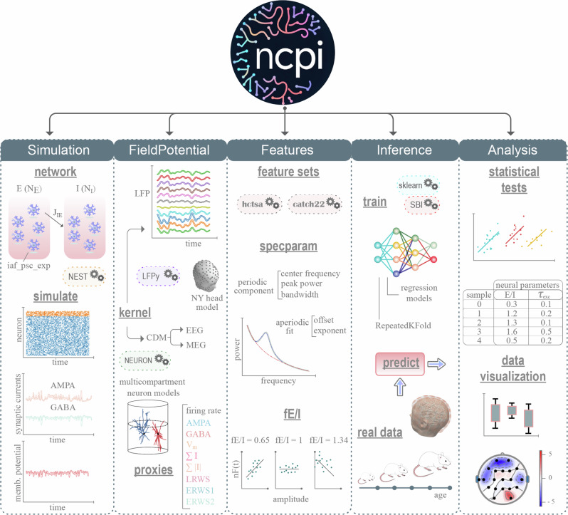
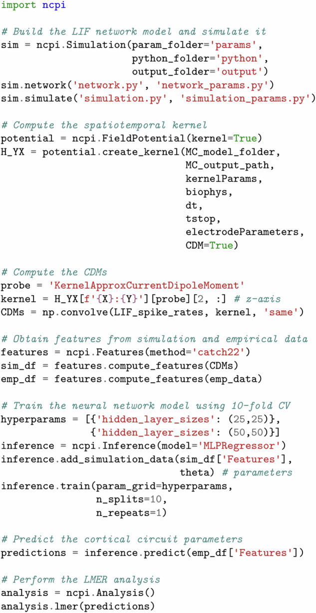
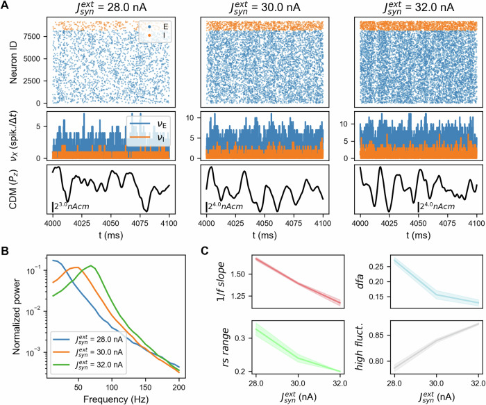
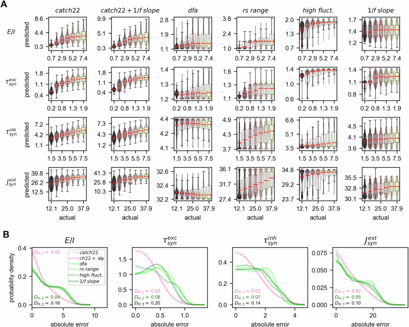
Computational research tools have reached a level of maturity that enables efficient simulation of neural activity across diverse scales. Concurrently, experimental neuroscience is experiencing an unprecedented scale of data generation. Despite these advancements, our understanding of the precise mechanistic relationship between neural recordings and key aspects of neural activity remains insufficient, including which specific features of electrophysiological population dynamics (i.e., putative biomarkers) best reflect properties of the underlying microcircuit configuration. We present ncpi, an open-source Python toolbox that serves as an all-in-one solution, effectively integrating well-established methods for both forward and inverse modeling of extracellular signals based on single-neuron network model simulations. Our tool serves as a benchmarking resource for model-driven interpretation of electrophysiological data and the evaluation of candidate biomarkers that plausibly index changes in neural circuit parameters. Using mouse LFP data and human EEG recordings, we demonstrate the potential of ncpi to uncover imbalances in neural circuit parameters during brain development and in Alzheimer's Disease.

Fig. 1. Outline of the ncpi toolbox.

The diagram shows the Python classes, their primary methods, and the included software libraries, and provides a representation of the processing flow. From left to right: simulation of neural activity, computation of field potentials, feature extraction, training of regression models, predictions computed on real data, and analysis and visualization of results. For further information, please refer to Methods.

Fig. 2. Python code snippet illustrating the use of the ncpi library and its classes.

This code snippet makes a few assumptions, such as the presence of ‘network.py’ and ‘simulation.py’ as files for creating and simulating the LIF network model, which are included in the ncpi library as examples, the availability of simulated firing rates as LIF_spike_rates, or the preprocessing of empirical data.

Fig. 3. Representative simulations illustrating the dynamics of the LIF network model in response to different external input values.

A Spike raster plots of the excitatory (E) and inhibitory (I) populations spanning 100 ms of spontaneous activity (top), spike counts in bins of width Δt (middle) and current dipole moment along the z-axis (P_z, bottom) for one of the six separate trials that were computed for this example. B Trial-averaged normalized power spectra of CDMs for the different values of external synaptic currents. C Features extracted from the CDMs across trials using the specparam library (1/f slope) and catch22 (dfa, rs range, and high fluctuation). For illustration, we focus on these three features from the catch22 subset, although we noted that most of the catch22 features exhibited marked trends in response to variations of the external input. A comprehensive description of the various catch22 features and their properties can be found in the associated publication.

Fig. 4. Comparison of features extracted from simulated signals.

Distributions of features computed on simulation data are shown as a function of synaptic parameters of the LIF network model (E/I, ${\tau }_{\mathit{syn}}^{\mathit{exc}}$, ${\tau }_{\mathit{syn}}^{\mathit{inh}}$ and $J_{\mathit{syn}}^{\mathit{ext}}$). Values of the parameters were binned into equal size intervals. In each bin, for a specific parameter, parameter values were within the limits of the bin, while the other synaptic parameters were free to vary without restriction. Each panel includes η² as a measure of effect size (ANOVA model).

Fig. 5. Predicted parameters generated from simulation data with various feature settings.

A Predicted versus actual values. B Probability functions of absolute errors. D_H,1 represents the Hellinger distance between the probability distributions of models trained with catch22 and catch22 + 1/f slope. D_H,2 represents the Hellinger distance between all the models trained on a single feature. D_H,3 represents the distance between catch22 and the models trained on a single feature. All prediction results shown here were computed on a held-out test dataset representing 10% of the whole simulation dataset.

Fig. 6. Predictions of changes in cortical circuit parameters derived from developmental LFP data.

Fits of parameters of the LIF network model (E/I, ${\tau }_{\mathit{syn}}^{\mathit{exc}}$, ${\tau }_{\mathit{syn}}^{\mathit{inh}}$ and $J_{\mathit{syn}}^{\mathit{ext}}$) were estimated using a MLP regressor based on the complete set of catch22 features (A) or the 1/f slope alone (B). The last column shows estimated normalized firing rates. Asterisks indicate significant differences between ages based on p-values obtained using the Holm-Bonferroni method with the LME and linear models defined in Eqs. 2 and 3 (see Methods). The significance levels are categorized as follows: a p-value between 0.01 and 0.05 is denoted by one asterisk (*), between 0.001 and 0.01 by two asterisks (**), between 0.0001 and 0.001 by three asterisks (***), less than 0.0001 by four asterisks (****), and p-values of 0.05 or greater are considered not significant (n.s.). To compute firing rates, 50 samples were drawn from each parameter prediction within the first and third quartiles of each age, and the firing rates were then normalized by the maximum firing rate of all samples.

Fig. 7. Predicted circuit parameter imbalances in AD based on EEG data.

Topographic representation of group differences in parameter fits based on the complete set of catch22 features (A) or the 1/f slope alone (B). The groups are classified as healthy controls (HCs), mild AD patients (ADMIL), moderate AD patients (ADMOD), and severe AD patients (ADSEV). Significant differences between groups were assessed using the Holm-Bonferroni method, applying the LME and linear models as defined in Eqs. 4–7. Only z-ratio values with an associated p-value ≤ 0.01 are plotted. The color range for the z-ratio values was selected such that positive differences relative to the control group were represented by shades of red, while negative differences were indicated by shades of blue.

References

1. D’Angelo, E. & Jirsa, V. The quest for multiscale brain modeling. Trends Neurosci.45, 777–790 (2022). - PubMed
1. Einevoll, G. T. et al. The scientific case for brain simulations. Neuron102, 735–744 (2019). - PubMed
1. Amunts, K. et al. The Human Brain Project-Synergy between neuroscience, computing, informatics, and brain-inspired technologies. PLoS Biol.17, e3000344 (2019). - PMC - PubMed
1. Madadi Asl, M., Valizadeh, A. & Tass, P. A. Decoupling of interacting neuronal populations by time-shifted stimulation through spike-timing-dependent plasticity. PLoS Comput. Biol.19, e1010853 (2023). - PMC - PubMed
1. Martínez-Cañada, P. et al. Combining aperiodic 1/f slopes and brain simulation: An EEG/MEG proxy marker of excitation/inhibition imbalance in Alzheimer’s disease. Alzheimer’s. Dement. Diagn. Assess. Dis. Monit.15, e12477 (2023). - PMC - PubMed
LinkOut - more resources