Low-Cost Hyperspectral Imaging in Macroalgae Monitoring

Abstract

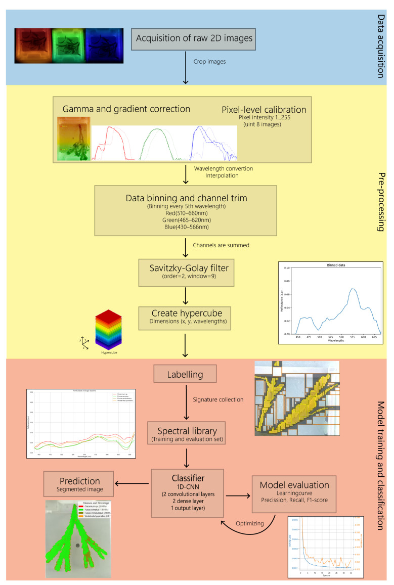
This study presents an approach to macroalgae monitoring using a cost-effective hyperspectral imaging (HSI) system and artificial intelligence (AI). Kelp beds are vital habitats and support nutrient cycling, making ongoing monitoring crucial amid environmental changes. HSI emerges as a powerful tool in this context, due to its ability to detect pigment-characteristic fingerprints that are often missed altogether by standard RGB cameras. Still, the high costs of these systems are a barrier to large-scale deployment for in situ monitoring. Here, we showcase the development of a cost-effective HSI setup that combines a GoPro camera with a continuous linear variable spectral bandpass filter. We empirically validate the operational capabilities through the analysis of two brown macroalgae, Fucus serratus and Fucus versiculosus, and two red macroalgae, Ceramium sp. and Vertebrata byssoides, in a controlled aquatic environment. Our HSI system successfully captured spectral information from the target species, which exhibit considerable similarity in morphology and spectral profile, making them difficult to differentiate using traditional RGB imaging. Using a one-dimensional convolutional neural network, we reached a high average classification precision, recall, and F1-score of 99.9%, 89.5%, and 94.4%, respectively, demonstrating the effectiveness of our custom low-cost HSI setup. This work paves the way to achieving large-scale and automated ecological monitoring.

Keywords: 1D convolutional neural network; artificial intelligence; biodiversity; classification; hyperspectral imaging; macroalgae; remote sensing; spectral analysis.

Figure 1

(A) Picture of the Hyperspectral Imaging (HSI) setup showing camera, optical system, continuous linear variable spectral bandpass filter (LVSBPF), aquarium with LED matrices. (B) Schematic diagram of the developed HSI system. A continuous linear variable spectral bandpass filter (LVSBPF) (red is 700 nm, blue is 400 nm) is mounted on a stepper motor linear stage and periodically translated in front of a consumer camera (GoPro Hero 11). An optical system (L₁–L₃) that implements an intermediate image plane at the filter and restricts the angle of incidence of the incoming light on the filter plane.

Figure 2

Gamma functions, i.e., digital intensity count versus normalized power (photon number), for each RGB channel of the GoPro camera: (a) red channel, measured with a 635 nm laser; (b) green channel, measured with a 520 nm laser; (c) blue channel, measured with a 405 nm laser. Max intensity at 255 Digital counts is indicated with a dashed point.

Figure 3

Spectrum of the laser pointers as measured (a) with a calibrated spectrometer and (b) with the Hyperspectral Imaging (HSI) camera.

Figure 4

Sampling area. (A) Geoposition of Hornbaek, Northern Zealand, Denmark. (B) The sampling site at Hornbaek Plantage, 56 05′31″ N, 12 29′10″ E. The red circle indicates the sampling area. (C) Photo of the sampling site.

Figure 5

Macroalgae samples collected at Hornbæk Plantage during April and July 2024.

Figure 6

Work-flow chart. The chart shows the simplified workflow for 1. The acquisition of the images. 2. The pre-processing part, which includes gamma and gradient correction of the RGB channel to uniform the color across the image, data binning, Savitzky-Golay filter and creation of hypercube. 3. Labelling data to create spectral library and training and classification of algae using the 1D Convolutional Neural Network model (1D-CNN).

Figure 7

Pre-processing of spectral data. (A) Spectral gradient from the LVSBPF. (Left) Gamma-corrected image at frame 40 of brown macroalgae with two red dots showing the pixel positions at the top and bottom of the grey-colored plate. (Right) The graph shows the spectrum for each channel (RGB) for the grey-colored plate. The solid line indicates the top part of the panel, and the dashed line indicates the bottom of the panel, showing the gradient shift between the top and bottom. The red arrows indicate the blue and red positions for the onset and are taken at the start of the blue spectrum and the end of the red spectrum. The spectra are normalized. (B) Shifted spectra. The graph shows the shifted spectrum for each channel (RGB) of the grey-colored plate after cross-correlation. The solid and dashed lines are described above. The spectra are normalized. (C) The red plot shows the normalized summed spectrum of trimmed RGB channels with linear interpolation of wavelengths. The Y-axis shows intensity measured in artificial units (a.u.) shown in red. The blue plot shows the same spectrum after pixel calibration, data binning (factor of 5), and the Savitzky–Golay filter (order = 2, window = 9) is applied. The Y-axis shows intensity measured in arbitrary units (a.u.) shown in blue.

Figure 8

Architecture of the 1D-CNN trained for macroalgal classification. Our CNN takes in spectral information from 45 bands from each pixel in the hypercube (violet, 400 nm and red, 700 nm) in the training set in the form of a one-dimensional array (1 × 45). The model consists of two convolutional layers, two pooling layers, one flatten layer, and two dense layers. The name of each layer is shown at the top, kernel numbers are shown underneath the convolutional and pooling layers, and kernel size is shown as k. Output size is shown on the side of each layer and at the bottom for the flatten and dense layer and output.

Figure 9

Mean reflectance spectra for each macroalgae class in the spectral library used as a training dataset for tuning the 1D-CNN model.

Figure 10

Classification results of each class generated by the 1D-CNN model. Predicted segmentation for (A) Ceramium sp., (B) Vertebrata byssoides, (C) Fucus serratus, and (D) Fucus versiculosus. The legend indicates the class and the corresponding coverage percentage predicted by the 1D-CNN model. For clarity, the background that represents the remaining coverage percentage is excluded.

References

1. Monserrat M., Comeau S., Verdura J., Alliouane S., Spennato G., Priouzeau F., Romero G., Mangialajo L. Climate change and species facilitation affect the recruitment of macroalgal marine forests. Sci. Rep. 2022;12:18103. doi: 10.1038/s41598-022-22845-2. - DOI - PMC - PubMed
1. Cheminée A., Sala E., Pastor J., Bodilis P., Thiriet P., Mangialajo L., Cottalorda J.M., Francour P. Nursery value of Cystoseira forests for Mediterranean rocky reef fishes. J. Exp. Mar. Biol. Ecol. 2013;442:70–79. doi: 10.1016/j.jembe.2013.02.003. - DOI
1. Krause-Jensen D., Duarte C.M. Substantial role of macroalgae in marine carbon sequestration. Nat. Geosci. 2016;9:737–742. doi: 10.1038/ngeo2790. - DOI
1. Basso D. Carbonate production by calcareous red algae and global change. Geodiversitas. 2012;34:13–33. doi: 10.5252/g2012n1a2. - DOI
1. Filbee-Dexter K., Wernberg T. Rise of Turfs: A New Battlefront for Globally Declining Kelp Forests. BioScience. 2018;68:64–76. doi: 10.1093/biosci/bix147. - DOI