Dopaminergic action prediction errors serve as a value-free teaching signal

Abstract

Choice behaviour of animals is characterized by two main tendencies: taking actions that led to rewards and repeating past actions^1,2. Theory suggests that these strategies may be reinforced by different types of dopaminergic teaching signals: reward prediction error to reinforce value-based associations and movement-based action prediction errors to reinforce value-free repetitive associations^3-6. Here we use an auditory discrimination task in mice to show that movement-related dopamine activity in the tail of the striatum encodes the hypothesized action prediction error signal. Causal manipulations reveal that this prediction error serves as a value-free teaching signal that supports learning by reinforcing repeated associations. Computational modelling and experiments demonstrate that action prediction errors alone cannot support reward-guided learning, but when paired with the reward prediction error circuitry they serve to consolidate stable sound-action associations in a value-free manner. Together we show that there are two types of dopaminergic prediction errors that work in tandem to support learning, each reinforcing different types of association in different striatal areas.

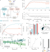
Fig. 1. TS is needed to facilitate learning and for execution of the auditory discrimination task.

a, Schematic of the task. Frequencies (freq.) represent auditory stimuli, volumes represent reward. b, Muscimol injection locations, indicated by the co-injection of fluorescent cholera toxin B. Scale bar, 2 mm. c, Psychometric task performance of mice, saline in TS (2 mice; 4 sessions), DMS (3 mice; 11 sessions) and TS (5 mice; 15 sessions). Lines represent logistic fits of the means. d, Schematic for inhibition of D1 SPNs or D2 SPNs. e, Psychometric task performance for opto-stimulated trials for the D1 (Drd1-cre) archaeorhodopsin (Arch) (8 mice; 15 sessions) and A2A (Adora2a-cre) Arch (8 mice; 12 sessions) mice. Lines represent logistic fits of the means. Stim, stimulation. f, Quantification of the bias for each session shown in e. Scatter dots represent the mean for each session, and error bars illustrate the variation of shuffled data (Methods). Colour-filled dots indicate P < 0.05. D1-Arch: P = 2.27 × 10⁻⁵, Cohen’s d = −1.40; A2A-Arch: P = 2 × 10⁻⁷, Cohen’s d = 2.33; Kruskal–Wallis test. g, Example lesion and control mice histology. h, Learning rate of the lesioned TS (n = 11 mice) and control (n = 10 mice) groups (lines represents group means). i,j, Maximum performance (i; P = 0.0023, Kruskal–Wallis test; Cohen’s d = −1.70) and maximum learning rate (j; P = 0.0006, Kruskal–Wallis test; Cohen’s d = −2.04) between the groups (same mice as in h). k, Example TH staining in the TS for control and lesion mice. l, Learning rate of the TS dopamine-ablated (n = 9 mice) and control (n = 5 mice) groups. m,n, Differences on the maximum performance (m; P = 0.006, Kruskal–Wallis test; Cohen’s d = −2.39) and maximum learning rate (n; P = 0.014, Kruskal–Wallis test; Cohen’s d = −1.71) between the groups (same mice as l). Error bars indicate s.d. in c,e,h,l. In box plots, boxes represent quartiles 2 and 3, the centre line shows the median and whiskers extend to the furthest data point within 1.5 times the inter-quartile range from the box. Source data

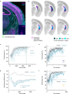
Fig. 2. TS dopamine release is correlated with contralateral movement.

a, Schematic of the experimental approach for recording dopamine activity in the VS and TS. The anterior–posterior distance between the VS and TS are not to scale. b, Fluorescent images showing optical fibre locations and dLight expression in the TS and the VS. Scale bar, 1 mm. c, Recording fibre locations from the VS and TS matched to the reference atlas. d, Example of a TS and a VS recording session aligned to time of leaving the centre port to make a contralateral (contra) choice or an ipsilateral (ipsi) choice. White dot shows time of entering contralateral or ipsilateral choice port. e, Average photometry traces in TS (n = 10 mice) and VS (n = 7 mice) aligned to task events. Shaded time windows show significant differences between the two trace types in each subplot, calculated by performing two-sample t-tests on 0.1-s bins and a P value threshold for significance of 0.01. f, Average response kernels to behavioural events for recordings in the TS and VS. Shaded time windows are calculated as in e. Coeff., coefficient. g, Percentage explained variance (var.) of the whole recording session (VS median = 31.3; TS median = 5.50) and for different behavioural kernels for linear regression models fitted on VS (n = 7 mice) and TS (n = 10 mice) recordings. Error bars represent s.e.m. in e,f. In box plots, boxes represent quartiles 2 and 3, the centre line shows the median and whiskers extend to the furthest data point within 1.5 times the inter-quartile range from the box. Source data

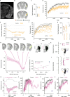
Fig. 3. TS dopamine release is consistent with encoding APE.

a, dLight recording in the VS. Each trace is the average of 200 trials. b, Example VS dopamine response size to contralateral cue binned every 40 trials. c, Average change in contralateral cue-aligned VS dopamine response. The solid orange represents the mean (n = 7 mice). The light orange trace is the mean predicted RPE response from 100 model agents. a.u., arbitrary units. d, Size of contralateral cue-aligned dopamine response in VS in the first and last session of training (n = 7 mice), P = 0.016 (paired two-sided t-test), Cohen’s d = −1.25. e–g, As a–c but for TS recordings (n = 6 mice). h, As d but for the TS (n = 9 mice), P = 0.006 (paired two-sided t-test). Cohen’s d = 1.19. i, Modelled responses for APE at the time of correct contralateral choice if the previous choice for that stimulus was ipsilateral or contralateral. j, As i but for an example average (mean) TS dopamine response. k, Regression coefficients. One-sided t-test against zero, corrected using the Bonferroni method for multiple comparisons. VS: n = 7 mice, P = 0.005, 1.0, 1.0, 1.0, 1.0 (left to right), (Cohen’s d = 2.23, 0.37, 0.23, 0.17, 0.13 (left to right)). TS: n = 6 mice, P = 0.04, 0.20, 0.20, 0.47, 0.63 (left to right), (Cohen’s d = −1.72, −1.13, −1.13, −0.84, −0.75 (left to right)). l,m, As i,j but for the VS response. n, Task design. WN, white noise. o, Modelled APE and RPE signals following the state change. p, Example TS dopamine responses to the contralateral choice in response to the normal or the white noise cue. q, TS dopamine response to the contralateral action before and after the introduction of the novel state (P = 0.01, paired two-sided t-test) (n = 6 mice), Cohen’s d = −1.81. r, As p but for a VS recording aligned to cue. s, As q but for VS recording aligned to cue. (P = 0.02, Wilcoxon signed-rank test) (n = 7 mice), Cohen’s d = 1.04. Error bars represent s.e.m. Source data

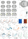
Fig. 4. TS dopamine release reinforces state–action associations.

a, Experimental approach. Slc6a3 encodes the dopamine transporter (DAT). b, Stimulation protocol. c, Average performance (mean) of mice. Left hemisphere n = 6 mice, right hemisphere n = 7 mice. Pre-stimulation data are pooled across all 13 recording sessions (n = 7 mice, 13 hemispheres). Error bars represent s.d. d, Distribution of session biases for the TS (4 mW n = 10 mice, n = 15 hemispheres, 8 mW n = 7 mice, n = 13 hemispheres) and the VS (4 mW n = 8 mice, n = 11 hemispheres, 8 mW n = 5 mice, n = 8 hemispheres) stimulations of the state–action experiment. TS: 4 mW P = 0.018, Cohen’s d = 1.46; 8 mW P < 0.001, Cohen’s d = 2.07. VS: 4 mW P = 0.57, Cohen’s d = −0.19; 8 mW P = 0.742, Cohen’s d = 0.19; Wilcoxon signed-rank test relative to zero (two-sided). e, Stimulation protocol. f, Same as d for the state–outcome TS-stimulation experiment (TS: 4 mW n = 10 mice, 8 mW n = 6 mice; TS: 4 mW P = 0.625, Cohen’s d = 0.40; 8 mW, P = 0.909, Cohen’s d = 0.05; VS: 4 mW P = 0.84, Cohen’s d = −0.21; 8 mW P = 0.461, Cohen’s d = 0.27; Wilcoxon signed-rank test relative to zero (two-sided)). g, Experimental approach. h, Average change in the bias for trials preceded by small or large dopamine choice movement responses (DA) in TS (n = 4, mice), error bars represent 68% confidence interval. i, Regression coefficients from a logistic regression (n = 4 mice) (log uncertainty: P = 0.006, Cohen’s d = 3.31; dopamine: P = 0.03, Cohen’s d = 2.01; one-sample t-test against zero, two-sided t-test). Filled circles represent significant correlations. Error bars represent s.d. j, As h but for VS dopamine responses (n = 5 mice). Error bars represent 68% confidence interval. k, As i but for VS dopamine at time of choice. n = 5 mice. log uncertainty: P = 0.03, Cohen’s d = 1.44; dopamine (at time of cue): P = 0.29, Cohen’s d = −0.54; one-sample t-test against zero, two-sided t-test. Error bars represent s.d. l, Example trajectories with smallest or largest Fréchet distances. m, Regression coefficients. Filled circles represent significant correlations for individual mice (n = 6 mice). One-sample t-test against zero, P = 0.03, Cohen’s d = −1.24. Error bars represent 95% confidence interval. In box plots, boxes represent quartiles 2 and 3, the centre line shows the median and whiskers extend to the furthest data point within 1.5 times the inter-quartile range from the box. Source data

Fig. 5. A dual-controller model predicts the effect of experimental manipulations.

a, Schematic of the network model. b, Top, task performance across learning for the full dual-controller model (combined), the value-based controller, or the value-free controller. Bottom, differences in performance between the combined model and the value-based model (12 random agents selected for each). c, Change of the model weights for a reward association (high tone→left action), as means for 100 agents. Vertical lines indicate inactivation time points in d. d, Performance levels before and after (as the mean after ten trials) model inactivations of the TS or the actor networks. e, Schematic of the experimental approach for acute inhibition of D1 SPNs or D2 SPNs in the TS. f, Quantification of the contralateral bias on opto-stimulated trials (Methods) for each session as a function of session’s performance. Error bars represent 95% confidence intervals. Lines show the mean and s.d. of linear fits for each mouse in each dataset. D1-Arch P = 0.004; A2A-Arch P = 7.6 × 10⁻⁴;  Methods; n = 8 mice. g, Proportion of significantly biased sessions in f as a function of performance. h, Final weights in the TS for each sound–action association. Source data

Extended Data Fig. 1. Task details and Optoinhibition histology.

a, Schematic of the task, left. Example spectrograms showing low (left plot) and high (right plot) “cloud of tone” stimuli. b, Coronal sections along the striatum indicating fiber placement positions (tip of the fiber). Note that fibers were inserted in both hemispheres and are mirrored here for illustration purposes. Primary auditory cortex (AUDp) projections (yellow) and primary somatosensory cortex (SSp) projections (blue) are shown in the other hemisphere. c, Horizontal (top) and side view (bottom) of the same histological data. For the horizontal section the recording location depths are collapsed onto a single horizontal atlas image for illustrative purposes. On the side view, the striatum is outlined and the AUDp projections are indicated in grayscale. All error bars represent the standard deviation.

Extended Data Fig. 2. Histology and quantification of TS lesions.

a, Representative image of a lesioned brain illustrating the image analysis used to quantify the proportion of lesioned striatum. Slices were registered to the atlas and the area with remaining neurons (as stained by NeuN) was defined. The rest of the striatum was considered as lesioned. b, Quantification of the lesion area for the 11 mice in the caspase dataset, across several coronal slices of the posterior striatum, that include the entire TS. c, Learning rate (performance vs. trial number) of individual mice in the lesion in TS and the control groups. Light blue and light gray traces are from mice that had an initial bias. d, Differences of means in performance between control and lesion groups. Dotted lines indicate the 95% confidence interval for the shuffled data (see methods). e, Learning rate for trials with the low tone stimulus (performance vs. trial number) of lesion TS and the control groups (shaded area indicates standard deviation). f, Same as F but for high tone stimulus trials (shaded area indicates standard deviation). Source data

Extended Data Fig. 3. Learning effects of D-AP5 infusions and the histology of TS-dopamine ablated mice and task response parameters.

a, Representative image showing the location of an infusion cannula implanted over the TS. b, Coronal sections along the striatum indicating cannula placement positions (center tip of the cannula). Note that cannulas were inserted in both hemispheres and are mirrored here for illustration purposes. Primary auditory cortex projections are also shown (yellow). c, Behavioral effect of acute D-AP5 infusion in expert mice (>5000 trials). n = 4 mice. d, Learning rate (performance vs. trial number) of D-AP5 and saline infusion groups (shaded area indicates standard deviation). D-AP5 n = 7 mice, Control n = 5 mice. e, Differences in performance between the groups. Dotted lines indicate the 95% confidence interval for the shuffled data (see methods). f, Same as D but showing the data from individual mice. g, Behavioral performance of mice in the last session of chronic D-AP5 infusion (brown), or when saline was infused in the first session after reaching 3000 trials, D-AP5 group (yellow) or the control group (gray). h, Quantification of the TH staining fluorescence ratio between the striatum and the cortex after background subtraction, at different levels in the allen reference (ARA) anterior-posterior axis. The data is shown as the fluorescence relative to controls. Primary auditory cortex projections are shown. i, Example TH-stained (dopamine axons) coronal slices at the level of the dorsal striatum (DS) for control and lesion mice. j, Correlation between the maximum performance achieved for each mouse and the lesion size (p = 0.049, two-sided Wald test). k, Time elapsed between center port poke and side port pokes, as medians for each animal, for the 6-OHDA and control groups (p = 0.31, Kruskal-Wallis test). l, Time elapsed between trials, as medians for each animal, for the 6-OHDA and control groups (p = 0.73, Kruskal-Wallis test). m, Differences of means in performance between control and lesion groups (6-OHDA n = 9 mice, Control n = 5 mice. Dotted lines indicate the 95% confidence interval for the shuffled data (see methods). n, Learning rate (performance vs. trial number) of individual mice in the 6-OHDA and the control groups (same mice as panel m). o, Learning rate for trials with the low tone stimulus (performance vs. trial number) of 6-OHDA and the control groups (same mice as panel m, shaded area indicates standard deviation). p, Same as O but for high tone stimulus trials. All boxplots show the range from quartile (Q1 - Q3), the median and the whiskers extend to the farthest data point lying within 1.5x the inter-quartile range (IQR) from the box. Source data

Extended Data Fig. 4. Histology and characterization of the photometry responses.

a, Coronal sections along the striatum indicating fiber placement positions (center tip of the fiber). Note that fibers were inserted in both hemispheres and are mirrored here for illustration purposes. Primary auditory cortex projections are shown in the other hemisphere. b, Horizontal (top) and side view (bottom) of the same histological data. For the horizontal section the recording location depths are collapsed onto a single horizontal atlas image for illustrative purposes. On the side view, the striatum is outlined and the AUDp projections are indicated in grayscale. c, Average photometry traces from TS (blue, n=10mice) and VS (orange, n = 7 mice) aligned to cue early in training (first three recorded sessions). Performance in these sessions was between 52.8% to 75.8% with an average performance of 64.0%. For TS mice it was comparable to VS mice (TS: min: 51.4%, max: 80.0%, avg: 64.5%; VS: min: 55.8%, max: 70.1%, avg: 63.3%). d, Same as C but aligned to contralateral choice. Movement initiation for choice (leaving the center port) occurs on average (0.19 s +/- 0.05 s) after cue onset. e, Same as C but aligned to reward delivery. f, Example of a TS (blue) and VS (orange) recording session aligned to cues predicting a contralateral choice. g, Comparison of rise time for dopamine response from onset of the cue in the VS (n = 7) and TS (n = 10) early in training (first three recorded sessions). Rise time onset is determined by the time taken for the dopamine trace to reach more than one standard deviation above a baseline period (1.5 s prior to cue onset) (p = 0.002 two-sided independent samples t-test), Cohen’s d = 1.90. h, TS dopamine responses for contralateral and ipsilateral choices aligned to movement onset early in training (first three recorded sessions). Shown separately for mice for whom contra-choice corresponded to high frequencies (n = 6) or mice for whom the contra choice corresponded to the low frequencies (n = 4). i, Same as H but for VS recordings aligned to cue onset. Shown separately for mice for whom contra-choice corresponded to high frequencies (n = 2) or mice for whom the contra choice corresponded to the low frequencies (n = 5). (n = 7 mice). j, Average photometry trace across the first 3 recorded sessions early in training, for an example mouse aligned to leaving to the side ports to return to the center port. k, Same as J but an average of all mice (n = 10). l, Average regression kernels across mice (n = 10) for the return to center behavioral events. m, Percentage explained variance for different kernel regression models of TS dopamine. Original kernel regression model with only choice (center port exit): median = 5.1, original model including the return to center (ipsi and contra) behavioral events median = 7.1, original model only allowing photometry data for which there are behavioral events to be included in the explained variance calculation “+ trimming” median = 8.5, model with return events and trimming median = 10.3. For one session in the original regression there was no video recording, so this is why the ‘original’ explained variance is slightly different to that reported in the main figure, as this session was not included in this analysis. n, Average photometry traces from cDLS (n = 3 mice) aligned to choice. o, Same as N but aligned to reward. All error bars represent SEM. All boxplots show the range from quartile (Q1 - Q3), the median and the whiskers extend to the farthest data point lying within 1.5x the inter-quartile range (IQR) from the box. Source data

Extended Data Fig. 5. TS dopamine is related to movement, not cue.

a, Change in percentage of completed trials (where animals made a left or right choice after leaving the center port) in trials with a normal stimulus (tone) or silence trials (p = 0.23, paired two-sided t-test, Cohen’s d = 1.15). b, Average photometry traces of one mouse aligned to contralateral choice. c, As for B but an average across mice (n = 3 mice). d, Change in peak response to the contralateral choice if the associated cloud of tones is replaced with silence (p = 0.31, paired two-sided t-test, Cohen’s d = 0.79). e, The number of tone-contralateral action pairings or silence-contralateral action pairings that the mice experienced prior to the recordings in B-D, (p = 0.07, paired two-sided t-test, Cohen’s d = 2.10). f, Difference in average speed for tone and silence trials for TS mice (n = 3), (p = 0.28, paired t-test, Cohen’s d = 0.84). g, Difference in average turn angle for tone and silence trials for TS mice (n = 3), (p = 0.75, paired two-sided t-test, Cohen’s d = 0.21). h, Animals were allowed to move freely in a different arena to the training box whilst dLight signals were recorded from the TS. Inset: Head angle during a detected turn in the freely moving arena. Dark blue line represents the orientation of the head at the beginning of the turn. Light blue line shows head orientation 0.5 s later. i, Example photometry response in the TS to contralateral and ipsilateral turn onsets in the freely moving arena. j, As in I but averaged across animals (n = 3 mice). k, Example traces from a TS recording session in the frequency discrimination task separated by size of the response. l, Average turn angle for these quartiles plotted against quartile midpoint (example session). m, The plateau of the sigmoid for each trial turn angle vs the average peak size of the TS photometry signal per quartile based on the photometry signal (example session). n, Data from early in training (first three recorded sessions) is analyzed as shown in O and a regression slope fitted (TS: n = 18 (6 mice, 3 sessions), VS: n = 21 (7 mice, 3 sessions). The slopes of the regressions (averaged per mouse) were tested against zero (one sample two-sided t-test). The TS slopes were significantly greater than zero (p = 0.03, Cohen’s d = 1.20), whereas the VS slopes were not (p = 0.87, Cohen’s d = −0.06). o, Schematic of the task structure when sound indicating an upcoming contralateral trial was played as mice return to the center port in 51.66 +/− 0.04 % of trials. p, Average dopamine response aligned to sound played while mice returned to the center during early training (n = 6 mice). q, Same as p but aligned to contralateral choice. r, Average amplitude of dopamine response aligned to the sound and choice across mice (p = 0.0047, Cohen’s d = 1.97). Size of the sound response is significantly smaller than zero (p = 0.008793, one-sample one-sided t-test against zero). s, Same as P but ipsi- and contralateral returns are plotted separately and returns without concomitant cue are also shown. t, Difference in response size of returns shown in S (circles, p = 0.2945, one way ANOVA, n = 6 mice) and response sizes of mice when the cue is novel during the first training session (crosses, p = 0.2815, Kruskal Wallis test, n = 3 mice). u, Schematic of the arena where the high and low tone task sounds were played passively as the mice explored. Passive sounds responses were tested in mice that were at an early stage of training on the CoT task (average performance 60.6 +/− 6.4 % in n = 5 mice). v, Average dopamine response in the TS during contralateral movement in the 2AC task (dark blue) and during passive sound presentation in subsequent exploration (pale blue) (n = 5 mice). w, Average amplitude of choice aligned response in the task and of passive sound response during exploration across mice (p = 0.0092, paired t-test, Cohen’s d = 2.11). There is no significant response to the sound (p = 0.45, one-sample two-sided t-test against zero). x, Average dopamine response in the TS during contralateral movement in the 2AC task (dark blue) and during passive presentation of white noise in subsequent exploration (pale blue) (n = 3 mice). Mice had on average experienced 93 presentations +/- 3.30 of white noise as a task cue before these recordings, this is less than half than during the CoT state-change experiment (195 + /−35 trials). y, Average amplitude of choice aligned response in the task and of white noise response during exploration across mice (p = 0.02, paired t-test, Cohen’s d = 3.87). There is no significant response to the sound (p = 0.84, one-sample two-sided t-test against zero). All error bars represent SEM. Source data

Extended Data Fig. 6. APE model and tests.

a, The model comprises an actor that learns stimulus-action values and guides action choices, a critic that learns a value function that is used to calculate RPE. The RPE signal is broadcast to the actor and critic to update their respective value functions. A value-free system learns to predict actions from those taken in the past and updates its prediction using the difference between its prediction and the action taken (APE). APE and RPE equations are written with respect to time (t), as is common, for illustrative purposes. For the model equations we use dwell time in the state (k) to approximate temporal discounting, see methods. b, The Markov decision process used to model the task. c, Correlation between the turn angle and the size of the dopamine response in the TS for all trials in all sessions of an example mouse. d, Correlation between the average speed of an example mouse and the TS dopamine response for all trials in all sessions. e, Linear regression coefficients for speed and turn angle on single trial TS (n = 6 mice) dopamine responses for the first three sessions of training. Stats: one-sample two-sided t-test against zero, speed: (p = 0.448, Cohen’s d = −0.34), turn angle: (p = 0.033, Cohen’s d = 1.20). Filled circles represent significant correlations for individual mice. Error bars represent 95% confidence interval. f, Turn angle of an example mouse over the course of training, binned per 40 trials. g, Average speed during a choice of an example mouse over the course of training, binned per 40 trials. h, Linear regression coefficients for the effect of trial number on speed or turn angle at a single trial level (n = 6 mice). Stats: one-sample two-sided t-test against zero, speed: (p = 0.154, Cohen’s d = 0.68), turn angle: (p = 0.340, Cohen’s d = −0.43). Filled circles represent significant correlations for individual mice. Error bars represent 95% confidence interval. i, TS dopamine response, binned per 40 trials of an example mouse over the course of training (blue). A linear regression model was built using average speed and turn angle to predict the TS dopamine signal. The model prediction from just the movement parameters over the course of training is shown in gold (binned per 40 trials). j, The movement model used in panel I was subtracted per trial from the TS dopamine responses to give the remaining signal that was not explained by speed or turn angle (residuals in blue). A new linear regression model was built using log trial number to account for the remaining TS dopamine signal (purple). Both are shown binned per 40 trials. k, The correlation between the individual trial residual dopamine responses and log trial number for an example mouse. l, Regression coefficients for the effect of log trial number on the residual dopamine response (n = 6 mice) (filled circles show significant correlations for individual mice). One-sample two-sided t-test against 0, p = 0.003, Cohen’s d = −2.14. Error bars represent 95% confidence interval. m, Total model variance explained by each parameter in a model where speed, turn angle and trial number are used to predict the size of the TS (n = 6 mice) dopamine response throughout learning. n, Difference between TS dopamine response in the last 40 trials of a previous session and next 40 trials of a session (between sessions) and first 40 trials of a session and last 40 trials of the same session (within session) (n = 6, between sessions: p = 0.27 one-sample two-sided t-test against 0, two-sided t-test Cohen’s d = 0.51, turn angle p = 0.05 one sample t-test against 0 two-sided t-test, Cohen’s d = −1.07). Error bars represent 95% confidence interval. o, Performance in the 50 trials before and after the state change (n = 13 mice, p = 1.98×10-4 paired two-sided t-test, Cohen’s d = 1.46). p, Changes in turn angle before and after the state change (n = 13 mice, p = 0.85 two paired two-sided t-test, Cohen’s d =−0.08). q, Changes in average speed before and after the state change (n = 13 mice, p = 0.02 paired two-sided t-test, Cohen’s d = 1.42). r, Performance before and after state change at trial 150 (black dashed line) binned per 20 trials (n = 13). Green lines show mean, error bars represent sem, grey lines represent data from individual mice. s, Same as R but showing the response time following the state change. t, Same as R but showing the bias towards ipsilateral choices following the state change. u, behavioral bias towards the large reward port before and after the change in value. The last 50 trials from each block are used for analysis with blocks being a minimum of 70 trials (n = 10 mice, p = 0.002 paired two-sided t-test, Cohen’s d = 1.39). v, Percentage of trials where mice did not make a choice before and after the value change is introduced at trial 100 (black dashed line) binned per 20 trials (n = 10 mice). Green lines show mean, error bars represent sem, grey lines represent data from individual mice. w, Same as V but showing the change in performance. x, Same as V but showing the change in response time. y, Same as V but showing the change in choice bias over the course of the session. All boxplots show the range from quartile (Q1 - Q3), the median and the whiskers extend to the farthest data point lying within 1.5x the inter-quartile range (IQR) from the box. Source data

Extended Data Fig. 7. Response of TS and VS dopamine responses to value manipulations.

a, Schematic of the outcome manipulation task design. b, Modelled responses for how APE and RPE signals would respond to changes in reward outcome. c, Example TS response to omissions, normal sized and large rewards. d, Group data (n = 6 mice) for TS dopamine response size to omission, normal and large reward (p = 0.84, p = 0.54, paired two-sided t-test, adjusted using Bonferroni correction), (Cohen’s d: large > normal 0.40, normal > omission 0.57). e, Same as c but for a VS recording. f, Same as d but for VS recording (n = 7 mice, p = 3.16×10-6, p = 8.87×10-6, paired two-sided t-test, adjusted using Bonferroni correction), (Cohen’s d: large > normal 7.01, normal > omission 5.89). g, Schematic of the predicted value manipulation task design. h, Model predictions for changes in predicted outcome value. i, Example movement-aligned TS response when the relative value of the cues changed. j, Summary data showing the change in movement-aligned response in the TS for relative value changes (p = 0.26, paired two-sided t-test) (n = 5 mice), Cohen’s d = 0.58. k, Same as i but for the VS response aligned to cue. l, Same as j but for the VS response aligned to cue (p = 2.41×10-4, paired two-sided t-test) (n = 5 mice), Cohen’s d = 5.56. All error bars represent SEM. Source data

Extended Data Fig. 8. APE and RPE models.

a, Model predictions for how the different models of dopamine respond in the state change experiment. b, Model predictions for how the different models of dopamine respond in the cue value change experiment. c, Salience model dopamine signal aligned to time of high cue, low cue, and reward. Size of response to cues shown for 100 agents over training. d, Novelty model dopamine signal aligned to time of high cue, low cue, and reward. Size of response to cues shown for 100 agents over training. e, Movement model dopamine aligned to time of contralateral choice, ipsilateral choice, and reward. Size of response to contralateral choice shown for 100 agents over training.

Extended Data Fig. 9. Histology and effects of dopamine optostimulation.

a, Coronal sections along the striatum indicating fiber placement positions (center tip of the fiber). Note that fibers were inserted in both hemispheres and are mirrored here for illustration purposes. Primary auditory cortex projections are shown in the other hemisphere. b, Horizontal (top) and side view (bottom) of the same histological data. For the horizontal section the recording location depths are collapsed onto a single horizontal atlas image for illustrative purposes. On the side view, the striatum is outlined and the AUDp projections are indicated in grayscale. c, Psychometric curves for all 8 mW sessions where dopamine release was optogenetically stimulated in the TS at the time of choice (center port). d, Scatterplot showing that the stimulation choice bias develops over the course of a session (8 mW, p = 0.035; 4 mW, p = 0.006, linear regression). e, Model simulation of the state-action optogenetic experiment. The APE was unilaterally stimulated when the cue predicted a contralateral action. f, Quantification of the contralateral choice bias on stimulated trials when optogenetic stimulation in the TS was delivered on 15% of trials at the center port. session (4 mW, p = 0.67; 8 mW, p = 0.28, Kruskal-Wallis test); 4 mW: n = 9 mice, 18 hemispheres mice, 8 mW n = 7 mice, 13 hemispheres g, Experimental design: animals enter a central port (gray) to initiate trials and then choose between water and water + optogenetic stimulation of dopamine release in the TS by entering one of two side ports. h, Choice bias (n = 5 mice) for 4 Hz optogenetic stimulation (p = 0.99, t-test) or 20 Hz optogenetic stimulation (p = 0.49, t-test). Solid dots indicate mean ± SEM and transparent dots indicate single sessions from individual animals. i, Same as g but with a 50% probability of receiving a water reward at the choice ports. j, Same as h but with the probability of receiving a water reward at the choice ports reduced to 50%. (TS, p = 0.11; VS, p = 0.002 Cohen’s d = 1.80, t-test). All boxplots show the range from quartile (Q1 - Q3), the median and the whiskers extend to the farthest data point lying within 1.5x the inter-quartile range (IQR) from the box. Source data

Extended Data Fig. 10. Motor effects of dopamine stimulation.

a, Heatmaps showing the occupancy for different sides of an arena during a real-time place-preference experiment where each side of the arena is paired with optogenetic stimulation of dopamine release in the TS. b, Bar graphs (mean) showing the percentage occupancy during control, stimulation in the left or in the right chamber. error bars represent SEM. c, Schematic showing the experimental closed-loop setup for detecting immobility and triggering dopamine release. d, Speed heatmap of trials sorted by movement onset for stimulated and control trials (n = 9 biologically independent animals). e, Speed histogram, same data as in n; error bars: SEM. f, g, h, i, Distribution, as means per mouse, of different movement parameters (see methods) (p:4 mW p = 0.21, 8 mW p = 0.42; q: 4 mW p = 0.67, 8 mW p = 0.78; r: 4 mW p = 0.87, 8 mW p = 0.80; s: 4 mW p = 0.93, 8 mW p = 0.50; paired two-sided t-test); same animals as in n. j, Regression coefficients for effect of TS dopamine response on the current trial on difference between turn angle on current and subsequent trial. Filled circles represent significant correlations for individual mice (n = 6 mice). Stats: one-sample t-test against zero, p = 0.07, Cohen’s d = −0.94. Error bars represent 95% confidence interval. Source data

Extended Data Fig. 11. Network model parameters and summary.

a, Moment in learning in which differences in between groups become significant, for the behavioral data and the network model. Dotted lines indicate the 95% confidence interval for the shuffled data (see methods). b, Change of the model weights during learning, as means for 100 agents, for the Critic, Actor, and TS networks. c, Summary schematic of the anatomical representation for the dual-controller model. Dotted arrow indicates the proposed, but as yet unverified, broadcast of APEs to the dorsal striatum. Source data

Extended Data Fig. 12. Response of TS dopamine to threat and movement.

a, Schematic of the experimental approach for recording dopamine activity in TS. b, Schematic of the experimental arena containing a threat zone (indicated by a dashed line) above which a looming stimulus can be displayed and a shelter (blue shaded area). c, Schematic of a single trial of the looming stimulus, consisting of 5 consecutive expanding spots. Black line illustrates how the looming spot radius changes over time. d, The dlight1.1 photometry traces for all three trials for each mouse (gray lines) and the average (blue line) in response to the five looming stimuli (top). The position tracks for each trial of the mice along the long axis of the behavioral arena (bottom). Looming spot onsets (black, dashed lines) and their durations (black circles) are shown. (n = 4 mice). e, Schematic of the frequency discrimination task. f, Average photometry response of the same mice as shown in (D) in the frequency discrimination task aligned to choice (n = 4 mice). g, Same as F aligned to reward. All error bars represent SEM. Source data

References

1. Wood, W. & Runger, D. Psychology of habit. Annu. Rev. Psychol.67, 289–314 (2016). - PubMed
1. Thorndike, E. L. Animal Intelligence: Experimental Studies (MacMillan, 1911).
1. Schultz, W., Dayan, P. & Montague, P. R. A neural substrate of prediction and reward. Science275, 1593–1599 (1997). - PubMed
1. Miller, K. J., Shenhav, A. & Ludvig, E. A. Habits without values. Psychol. Rev.126, 292–311 (2019). - PMC - PubMed
1. Lindsey, J. & Litwin-Kumar, A. Action-modulated midbrain dopamine activity arises from distributed control policies. NeurIPS 2022 Conferencehttps://dl.acm.org/doi/10.5555/3600270.3600670 (2022). - DOI
LinkOut - more resources