Digitalized organoids: integrated pipeline for high-speed 3D analysis of organoid structures using multilevel segmentation and cellular topology

Abstract

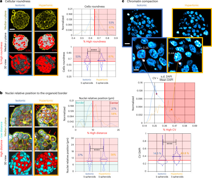
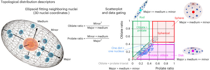
Organoids replicate tissue architecture and function and offer a unique opportunity to explore the impact of external perturbations in vitro. However, conducting large-scale screening procedures to investigate the effects of various stresses on cellular morphology and topology in these systems poses important challenges, including limitations in high-resolution three-dimensional (3D) imaging and accessible 3D analysis platforms. In this study, we introduce an AI-based multilevel segmentation and cellular topology pipeline for screening morphology and topology modifications in 3D cell culture at both the nuclear and cytoplasmic levels, as well as at the whole-organoid scale. We demonstrate the versatility of our approach through proof-of-concept experiments, encompassing well-characterized conditions and poorly explored mechanical stressors such as microgravity. By offering a user-friendly interface named 3DCellScope and a comprehensive set of tools for discovery-like assays in screening 3D organoid models, our pipeline demonstrates wide-ranging potential for applications in biomedical research.

Fig. 1. ‘Digitalized’ organoids principle.

a, Schematic depicting the pipeline. Top, Organoids were imaged using 3D fluorescence microscopy. Middle, The complete 3D digitalization of organoids consists of three layers of segmentation. Bottom, The resulting data are understandable through data mining. b, Nuclei and cell segmentation applied on a primary PDAC organoid. The white arrows indicate low-intensity nuclei.

Fig. 2. Interactivity and data navigation through three levels of 3D segmentation, graphical filtering and image feedback.

a, 2D and 3D visualization of cancer cell spheroids (HCT116), labeled with phalloidin and DAPI. 3D cell contours (middle) and 3D nuclei contours with organoid contours (bottom) are shown. Scale bar, 60 µm. b, Graphical display and gating on a histoplot (top). Manual filtering (red bar) can be adjusted to exclude small objects, with feedback provided on segmented or raw images (right). The bottom plot shows the mean nuclei volume obtained after filtering (gray line for standard error) versus the number of cells per organoid for the four organoids. Scale bar, 15 µm. c, Schematic and histoplot of nuclei centroid distance from the organoid’s border. Plot depicts filtering in two classes: nuclei within 0 µm to 20 µm (green–cyan) and nuclei at a distance greater than 20 µm (red). d, 2D and 3D visualization of nuclei gating based on their distance to the organoid border. Plot shows the mean (±s.e.m.) nuclei volume for two classes: external (<10 µm from the border) and internal (>10 µm; n = 895).****P < 0.0001, using a two-tailed unpaired t-test with Welch’s correction. Scale bar, 30 µm. Source data

Fig. 3. Proof-of-concept experiment on well-known conditions of morphological modifications to validate multi-scale morphological parameters.

a, Cell roundness was compared under isotonic and hypertonic conditions. Representative actin images are shown. The cell roundness of two representative spheroids (one per condition) are plotted in the histoplot, and filtering was applied using the normalized histoplot with a red bar indicating a high cell roundness threshold. The percentages of cells exhibiting high roundness are displayed (red) on 2D and 3D segmentation. Scale bar, 30 µm. Red arrows highlight cells of high roundness in the core of the spheroid. Violin plots show the cell roundness for isotonic and hypertonic conditions. b, The relative position of nuclei to the organoid border was compared between isotonic and hypertonic conditions. Representative images with DAPI and phalloidin staining are displayed, with cyan contours representing nuclei near the border and red contours marking nuclei farther from the border. Filtering was applied to classify nuclei into two groups based on their relative position to the organoid border. Red arrows point to nuclei in the long-distance class. Scale bar, 10 µm. The histoplot presents the relative position of nuclei for two representative spheroids (one per condition), while the violin plots show the distribution of nuclei positions for five spheroids per condition. c, Chromatin compaction was evaluated by the CV of DAPI staining under isotonic and hypertonic conditions. Clickable nuclei contours, marked by red dots and white hands, link the images to the corresponding histoplot (two spheroids represented, one per condition). Filtering was applied to identify nuclei with high CV values. Violin plots show the distribution of CV values for both conditions. For all violin plots, mean values are represented by blue bars. ****P < 0.0001, using a two-tailed unpaired t-test with Welch’s correction; analysis based on ten organoids (five organoids per condition). Scale bars, 15 µm and 5 µm (zoomed images). Source data

Fig. 4. Topological distribution descriptors.

Schematic representation of ellipsoid fitting around neighboring nuclei, displaying ellipsoid axes and calculation of oblate and prolate ratios. Scatterplot illustrates the relationship between oblate and prolate ratios, with multi-class gating description (each dot represents one nucleus). Source data

Fig. 5. Analysis of 3D topology and comparison of microniche shapes in a complex organoid environment.

a, Comparison of cellular positioning on two different shapes of microniche (blue, ‘cup’; orange, ‘well’) and microniche without ECM (yellow) depicted on a scatterplot of oblate-versus-prolate ratio (one dot denotes one nucleus). Color-coded feedback (red contours denote ‘spherical’ gate, cyan denotes all other nuclei) presented on 3D segmentation views (xy and xz) and a median xy plane (indicated by white double arrows) with the percentage of nuclei exhibiting ‘spherical’ ellipsoids for each microniche (representing an isotropic neighborhood). Red arrows indicate disorganized multilayers of cells. Scale bar, 25 µm. b, Comparison of different regions of interest within a complex primary PDAC organoid. Two complementary strategies were used: a single-step data gating on the scatterplot of oblate-versus-prolate ratio, enabling feedback of three different classes—disk (magenta), rod (green) and sphere (red)—on the 3D view. Red arrows denote enriched areas of ‘sphere’ nuclei distribution (in the core of the organoid), while green arrows highlight ‘rod’ enriched areas (in several buds). ‘Disk’ (magenta) nuclei distribution is not displayed in zoomed images for improved visualization. A two-step strategy is also applied, starting with image gating on segmented images (image gating: core (red), bud (light blue/cyan), borders (orange), with corresponding nuclei counts displayed). Subsequently, the same data gating step (magenta/green/red) is applied to multi-region scatterplots. Additionally, linear regression analysis is performed, and corresponding slope values are presented. Pie charts display the corresponding nuclei percentage in each data gate (disk, rod and sphere) per image gate (regions of interest: core, bud and border). Scale bars, 150 µm. Source data

Fig. 6. Integrated workflow for 3D morphological signature understanding.

a, 3D imaging screening generated 120 organoids under four conditions (day 0: GC and F, day+1: GC24 and F24). Morphological features across 8,215 cells were amalgamated without condition descriptors. b, This ‘blind’ pool is used for unsupervised PCA to reduce data’s dimensionality. The cells, now identified by their respective conditions, were then plotted based on their PC1 values. Subsequent clustering isolated specific cell populations based on distinct signatures. Violin plots represent unsupervised clustering of PC1, illustrating cell volume differences. c, Image feedback showcased a prevalent localization of the ‘high PC1’ population (red) at the organoid border. Scale bar, 50 µm. d, Biologically meaningful gating based on the distance from the organoid’s border was applied. Plots of guided filtering on nuclei distance to the border with significant cell volume differences. For all violin plots, blue bars indicate the mean. ****P < 0.0001, using a two-tailed unpaired t-test with Welch’s correction.

Extended Data Fig. 1. Scheme of preprocessing, segmentation processes and final results with features extracted.

The pipeline starts from (1) optional preprocessing, for example, histogram matching to correct intensity loss due to depth penetration. The preprocessed data is then resized to match the voxel size of 3D StarDist training data. (2) Nuclei are segmented with an AI Stardist pre-trained network (4 different CNNs available). (3) Organoid segmentation was performed using one of the channels or the channels mean, it consists of steps as follows: Enhance Local Contrast (CLAHE), Gaussian blur, Otsu threshold, Morphological operations, Keep largest object. (4) The segmented organoid mask is used for cleaning, that is, debris with centroids outside the organoid are removed and organoid/spheroid borders are dilated to secure the inclusion of all nuclei and cytoplasmic signals. (5) Cell segmentation was performed using seeded watershed based on nuclei segmentation and cell channel (nuclei are considered as seeds). The expansion of the cell watershed is limited to the organoid volume. The distance between a nucleus border and the corresponding cell border is constraint to a maximum value (i.e 14 µm). The label mask of cells is filtered with a 3D median filter.

Extended Data Fig. 2. Data import, export and interface of 3DCellScope.

a. Images imported into 3DCellScope for segmentation, user can run segmentation on selected image and the segmentation masks and csv files were output in results folder. b. Interface of 3DCellScope and steps to generate the results. (1) File management: Select images folder and choose image for visualization or processing. (2) Channel preprocessing: Add preprocessings for selected channels. (3) Nuclei segmentation: Select Stardist model and fit model resolution. (4) Organoid segmentation: Apply Otsu threshold or Dynamic Range threshold for organoid segmentation. (5) Cell segmentation: Run 3D watershed using intensity channel or distance map. (6) Process image: Click to start processing selected image. (7) Image/results visualization: Visualize the image and results in 2D and 3D view. (8) Data exploration: Explore data with various tools, such as generating plots, performing gating and running PCA.

Extended Data Fig. 3. Comparison of different Stardist models: DeepStar3D, Cellos, AnyStar and OpSeF.

a. 3D nucleus segmentation results using different Stardist models. The quantitative and qualitative comparison shows consistent performance of DeepStar3D across all benchmark datasets. N denotes nuclei count, F1 denotes F1 score over IoU50, scale bar: 30 µm. b. Spearman correlations (left) between IoU vs. SNR and IoU vs. Nuclei Density for each Stardist model on the ZeroG breast cancer spheroid. N.S for non significative P-value (=no correlation), using two-tailed t-test and overlay performance examples on low SNR image (right) of the 4 Stardist models, image from human colon organoid, scale bar: 15 µm. Source data

Extended Data Fig. 4. Quality assessment of cell segmentation.

a. Representative segmentation results of cells, based on Actin staining, of same spheroid at 3 different z-planes with examples of bad segmentation (‘false’ ROI = blue dots) and percentage of mis-segmentation (% errors) are provided for each images (see online for details on % errors calculation). Grey dotted-lines = coverslip position, yellow lines = imaging plan. Scale bar = 25 µm. b. Similar as a but from 6 different spheroids at the same depth (70 µm) with corresponding mean of percentage errors. Scale bar = 60 µm.

Extended Data Fig. 5. Example of interface to perform data mining.

(1) List of wells and conditions: Input data listed in terms of wells and conditions. (2) Feature list: Features can be imported and generated from multiple sources, for example, imported csv files, extraction from masks and images, feature calculator, normalization, Principal Component Analysis (PCA), classification (Support Vector Machine, Decision Tree, Random Forest Algorithms) etc. Feature calculator for creating new feature is shown in the zoom-in view. (3) Selection: Selection window shows properties of selected object. Properties shown include sample, well, condition, field and all measurements. (4) Plot views: Multiple types of graphs can be created, for example, cell level plot (Histogram, scatter plot, bubble plot), well/sample plot (Bar plot, scatter plot, bubble plot), plate/batch level plot (Heat map, batch vs. batch scatter plot). (5) Gates: Gates can be created on histograms and scatter plots, instant feedback is shown in image views while adjusting gating threshold. (6) Image views: Image views show channels, masks and gates. Object can be selected interactively in 2D or 3D or plot view. (7) 3D rendering: Fast 3D rendering based on input parameters of max 3D resolution and z spacing.

Extended Data Fig. 6. Summary of 3D topological descriptors.

a. Nuclei spatial arrangement descriptors: Cell-to-Neighborhood: An ellipsoid fitted from all nuclei coordinates in a spheroid of radius r (µm) provides various descriptors (listed in the table). b. Nuclei density descriptors: Cell-to-Cell: Illustrations showing Ripley nuclei and crystal distance definition. Ripley nuclei can be estimated by multiplying the number of nuclei inside the sphere of radius r µm with the ratio of sphere volume to organoid volume inside the sphere. Crystal distance is defined as the grid spacing assuming equal 3D repartition of nuclei in the spheroid. The full list of nuclei density descriptors is shown in the corresponding table.

References

1. Stylianou, E. et al. A mathematical model for the role of cell accumulation in age-related intestinal tumorigenesis. PLoS ONE11, e0149562 (2016).
1. Yin, J. et al. Mechanical forces contribute to aged-related joint degeneration. JCI Insight5, e132351 (2020).
1. van den Berg, C. W. et al. Renal subcapsular transplantation of PSC-derived kidney organoids induces neo-vasculogenesis and significant glomerular and tubular maturation in vivo. Stem Cell Rep.10, 751–765 (2018). - PMC - PubMed
1. Drost, J. & Clevers, H. Organoids in cancer research. Nat. Rev. Cancer18, 407–418 (2018). - PubMed
1. Rossi, G., Manfrin, A. & Lutolf, M. P. Progress and potential in organoid research. Nat. Rev. Genet.19, 671–687 (2018). - PubMed
MeSH terms
LinkOut - more resources