Repeatability of evolution and genomic predictions of temperature adaptation in seed beetles

Abstract

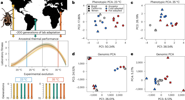
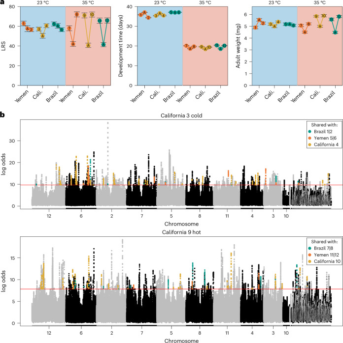
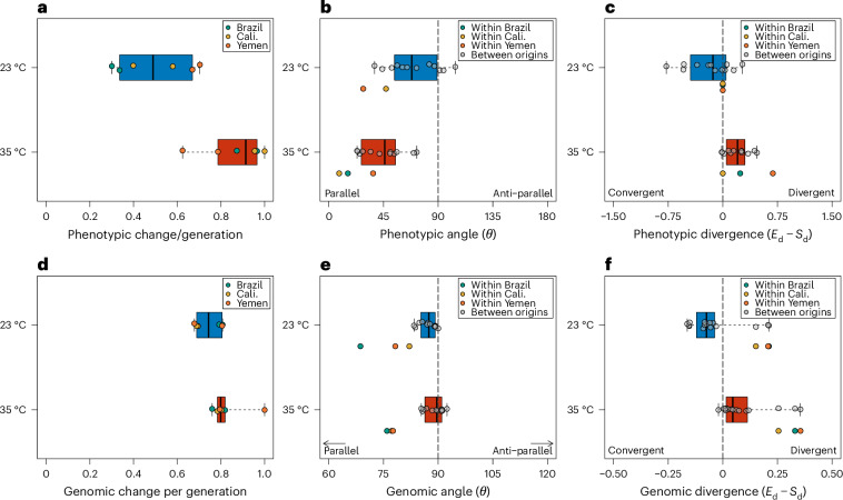
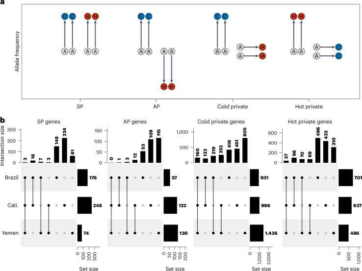
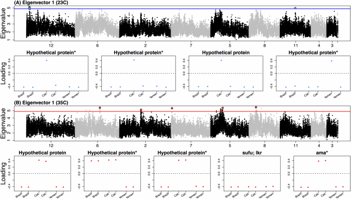
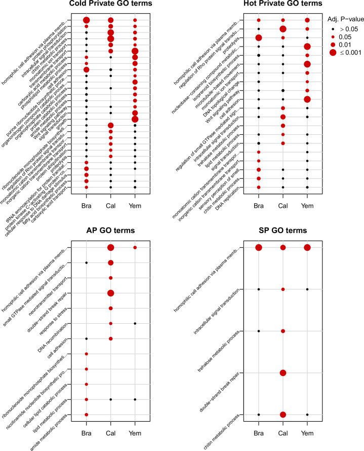
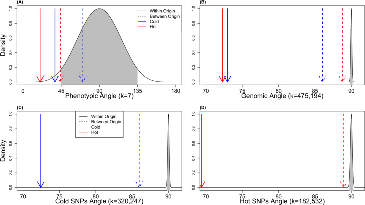
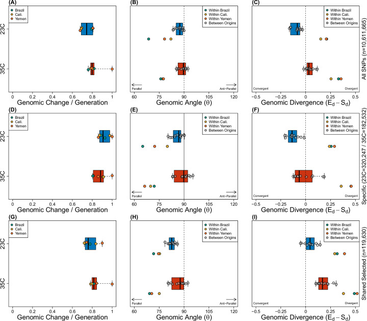
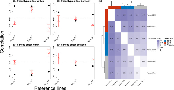
Climate warming is threatening biodiversity by increasing temperatures beyond the optima of many ectotherms. Owing to the inherent non-linear relationship between temperature and the rate of cellular processes, such shifts towards hot temperature are predicted to impose stronger selection compared with corresponding shifts towards cold temperature. This suggests that when adaptation to warming occurs, it should be relatively rapid and predictable. Here we tested this hypothesis from the level of single-nucleotide polymorphisms to life-history traits in the beetle Callosobruchus maculatus. We conducted an evolve-and-resequence experiment on three genetic backgrounds of the beetle reared at hot or cold temperature. Indeed, we find that phenotypic evolution was faster and more repeatable at hot temperature. However, at the genomic level, adaptation to heat was less repeatable when compared across genetic backgrounds. As a result, genomic predictions of phenotypic adaptation in populations exposed to hot temperature were accurate within, but not between, backgrounds. These results seem best explained by genetic redundancy and an increased importance of epistasis during adaptation to heat, and imply that the same mechanisms that exert strong selection and increase repeatability of phenotypic evolution at hot temperature reduce repeatability at the genomic level. Thus, predictions of adaptation in key phenotypes from genomic data may become increasingly difficult as climates warm.

Fig. 1. Experimental design.

a, Populations were collected from California (yellow), Brazil (teal) and Yemen (orange) and adapted to benign lab conditions (29 °C) for approximately 200 generations. Thermal performance curves (with 95% confidence intervals shown as shaded bands) of the three populations show the classic asymmetric shape and depict how population growth rate (adult offspring production/generation time) changes with temperature. While mean growth rates are slightly lower at 23 °C compared with 35 °C, the slope of the performance curve is steeper at temperatures higher than the optimum. To start experimental evolution, lines were placed at either 23 °C or 35 °C, with two replicates in each treatment per genetic background. Horizontal black bars in the arrows depicting each experimental evolution line indicate the time at which lines were sequenced. The sequencing of heat-adapted lines at generation 3 represent the genomic estimates of ancestral variation. b–e, For both the seven life-history phenotypes (b,c) and for all genomic SNPs (d,e), principal component analysis (PCA) summaries are presented of evolutionary change between ancestral (grey) and heat- (red) and cold-adapted (blue) lines. Phenotypes were measured in a common garden design including both the low and high temperature. The world map was generated using the R packages ggplot and maps. Scientific illustration of C. maculatus drawn by Milena Trabert.

Fig. 2. Phenotypic evolution and example of genomic data.

a, Means (±1 s.e.m.) are shown for ancestors (A) and evolved lines for three of the seven measured traits (see Extended Data Fig. 1 for all traits). Phenotypes of evolved lines (1–12) are shown only as measured in their local temperature regime (cold lines, 1–6, light blue shading, measured at 23 °C; hot lines, 7–12, light red shading, measured at 35 °C). Cali., California. b, Manhattan plots of rolling average log odds P values (window size = 20 SNPs) for one heat-adapted and one cold-adapted line from the California background (see Supplementary Fig. 1 for all populations) across all putatively selected sites (n = 475,194) using R package RcppRoll (v.0.3.0). The largest ten scaffolds (that is, chromosomes) are labelled. The 0.001th quantile of rolling average P values is given by the horizontal orange line for each line. SNPs whose rolling average P values are also above their respective 0.001th quantile in other populations are coloured. There is a clear polygenic signal of adaptation. Note that the California lines shown here exhibit many more SNPs in common with the single other California replicate (yellow points) than those shared with any of the four line replicates of different origin (teal and orange points).

Fig. 3. Evolutionary rates, pairwise angles and measurements of divergent evolution.

a–f, Distribution of all phenotypic and genomic evolutionary rates (a,d), pairwise angles (b,e) and measurements of convergent or divergent evolution (c,f) for cold (blue) and hot (red) lines are shown. Boxplots display the median (solid centre line), interquartile range (bounds of the box) and range (whiskers) of the data. All genomic estimates are based on the set of SNPs putatively under selection in any population (n = 475,194). Angles and divergences are given for pairwise comparisons between lines of different (grey points) and same (coloured points) genetic background. Angles of 0° represent completely parallel responses, while angles of 90° represent uncorrelated responses. Divergence was calculated as the difference in Euclidean distance between population pairs at the end (E_d) and start (S_d) of experimental evolution, and are divergent when the distance between end points is greater than the distance between start points (E_d − S_d > 0), or convergent if the opposite is true (E_d − S_d < 0). Evolutionary rates have been scaled by the maximum evolutionary rate in the dataset, while divergences have been scaled relative to the distance between the two most differentiated ancestors. Inestimable phenotypic angles due to sampling error are not shown (within Brazil, 23 °C).

Fig. 4. The criteria for allele classifications and overlapping gene sets of those alleles.

a, Schematic showing how SNP and gene classes were assigned based on patterns of allele frequency change from the ancestor (A) to the evolved cold (C) and hot (H) lines. For each class, we require both replicates of a particular background to behave similarly (that is, more extreme than the 1st or 99th percentiles with the same direction of allele frequency change in both replicates). The four classes identified are: (1) synergistically pleiotropic (SP) SNPs, which are selected for in the same direction between regimes; (2) antagonistically pleiotropic (AP) SNPs, which are selected in opposite directions between regimes; (3) private cold SNPs, which are selected for only in the cold regime; and (4) private hot SNPs, which are selected for only in the hot regime. b, Upset plots of gene sets based on corresponding SNP set classes (Extended Data Fig. 2) located in protein-coding regions. There is significant excess of shared private selection genes, and more gene sharing among genetic backgrounds adapting to cold temperature.

Fig. 5. A prediction of temperature-dependent epistasis for fitness based on thermodynamics of cellular processes.

For each plot, coloured vertical lines denote the temperature of our thermal regimes (23 °C and 35 °C). a, Reproductive rate increases exponentially with temperature at the colder range due to relaxation of thermodynamics constraints on enzymatic reactions, but starts to follow a pattern of diminishing returns at warmer temperatures due to ecological constraints placing limits on reproductive output. Illustrated for three hypothetical genetic backgrounds (purple, brown and pink) with wild types (solid lines) and a mutant (dashed lines, whose selection coefficient is denoted by s) with a 10% increase in enzymatic reaction rate at 23 °C. This results in strong selection on the mutation at cold temperature for all backgrounds as these are far from their optimal reproductive rate, but weak selection at hot temperature at which all backgrounds are close to the maximal achievable reproductive rate determined by ecological factors. Epistasis is weak and selection is similar across backgrounds at all temperatures. b, Warm temperatures increase a range of molecular failure rates, which results in less enzyme ready to catalyse reactions, and more misfolded proteins within cells, leading to protein toxicity and depressed fitness. Illustrated for three genetic backgrounds with stable (purple), intermediate (brown) and unstable (pink) wild-type protein. A mutation increasing stability (dashed lines) was introduced on each background. Selection on the mutation is weak at cold temperature for all backgrounds but can become very strong at hot temperatures depending on the wild-type protein stability, and strong epistasis for fitness results. c, Fitness, as the product of reproductive rate and molecular failure rate, is depicted for the wild type (black), and the mutants with increased enzymatic reaction rate (blue) and increased protein stability (red) for the pink background.

Fig. 6. Genomic predictors of phenotypic divergence and laboratory fitness at hot temperature (35 °C).

a–d, Genomic and phenotypic offsets were calculated using reference populations identified separately for each geographic origin. Within each origin, the line with the highest lifetime adult offspring production per generation (i.e. laboratory fitness) was designated as the reference population. Genomic offsets were calculated based on SNPs whose P values for allele frequency change fell within the top 0.001th quantile for each reference (n = 10,546–10,649). Relative fitness offsets were calculated as a line’s lifetime adult offspring production per generation time, relative to that of the reference population. Similarly, phenotypic divergence offsets were calculated as the Euclidean distance in scaled trait space to this reference population. Offsets are organized by predictions within genetic backgrounds (a,c) and between genetic backgrounds (b,d). Regression lines are dotted by the origin of the reference population, while symbol colours refer to ancestral (grey), cold (blue) and hot (red) lines. Genomic offsets predict maladaptation within a and c but not between b and d geographic origins.

Extended Data Fig. 1. Phenotypic evolution of 7 life-history traits.

Means and one standard error for the seven life-history traits in evolved and ancestral lines. Note that ancestors (‘A’) and evolved lines (1-12) were measured in their evolved temperature regime, denoted by background color.

Extended Data Fig. 2. Upset plots of different categories of allele frequency change among thermal regimes.

Cold Private (selected only at cold), Hot Private (selected only at hot), AP (antagonistically pleiotropic - selected in opposite directions in the hot and cold regime) and SP (Synergistically pleiotropic - selected in the same direction in the hot and cold regime).

Extended Data Fig. 3. Eigen analyses of genomic regions showing parallel regions of allele frequency change.

Manhattan plots showing the Eigenvalue for regions (window size = 200 SNPs) of the genome across all 6 cold-adapted (A) or hot-adapted (B) lines. Windows exceeding the 99% significance threshold are highlighted- all 4 independent chromosomal windows for 23 °C (below panel A) and the top 5 significant windows for 35 °C (below panel B). For each significant window (presented in left-to-right order), we show population loadings on Eigenvector 1, with genes in or nearest to each window labeled (nearest genes marked with asterisks).

Extended Data Fig. 4. Dot plot indicating significant GO terms per gene set category (based on Fig. 4).

Adjusted p-values equal to 1 are not shown.

Extended Data Fig. 5. Null distributions of random angles in k-dimensional space.

Distributions shown are associated with (A) phenotypic parallelism, (B) genomic parallelism using any selected site, and (C & D) genomic parallelism using sites selected for per regime. The 95% confidence intervals associated with random angles are shown shaded in grey. The mean within- and between-origin comparisons are presented as arrows and colored per temperature regime.

Extended Data Fig. 6. Evolutionary rates, pairwise angles, and measurements of divergent evolution between different selection criteria of SNPs.

Allele frequency changes found in all SNPs called (top row, “all”), SNPs selected for in each temperature regime independently (middle row, “specific”), and SNPs which are both selected for in any line but also polymorphic among all ancestors (bottom row, “shared”). Evolutionary rates (A & D & G) are given for individual lines, while angles (B & E & H) and divergences (C & F & I) are given for pairwise comparisons between populations of different (grey points) and same (colored points) genetic background. Evolutionary rates have been scaled by the maximum evolutionary rate in the dataset, while divergences have been scaled by the distance between the two most differentiated ancestors.

Extended Data Fig. 7. Bootstrapped correlations for genomic offsets at hot temperature using sets of randomly chosen SNPs.

Genomic offsets (A-D) were calculated 1,000 times using randomly sampled SNPs of equal number to the SNPs used in hot line offsets (n=10,546-10,649). The means and 0.025th and 0.975th quantiles for bootstrapped correlations are shown as colored points and lines, respectively. The correlation based on selected SNPs is shown as a solid black point (see Fig. 6). Correlations are separated by within (A, C) and between (B, D) origins. Predictions based on candidate SNPs outperform those based on randomly selected SNPs. Note that predictions based on random SNPs sometimes go in opposite direction to those based on selected SNPs (for example, see predictions within the Yemen background), yielding highly inaccurate predictions. This may happen when several isolated populations adapt to a particular environment (for example, heat) and experience stronger selection than populations evolving in another environment (for example, cold). When the case, the populations under stronger selection can show high phenotypic similarity but diverge more from each other at neutral sites due to stronger genetic drift and draft during the processes of adaptation. As a result, genomic distances (and offsets) based on neutral variation can be larger between populations adapting in parallel (illustrated by whole-genome FST for the Yemen background; E). Thus, sometimes the use of neutral or genome-wide variation may result in counterintuitive, and even misleading, predictions of local adaptation.

References

1. Lässig, M., Mustonen, V. & Walczak, A. M. Predicting evolution. Nat. Ecol. Evol.1, 0077 (2017). - PubMed
1. Blount, Z. D., Lenski, R. E. & Losos, J. B. Contingency and determinism in evolution: replaying life’s tape. Science362, eaam5979 (2018). - PubMed
1. Wortel, M. T. et al. Towards evolutionary predictions: current promises and challenges. Evol. Appl.16, 3–21 (2023). - PMC - PubMed
1. Storz, J. F. Causes of molecular convergence and parallelism in protein evolution. Nat. Rev. Genet.17, 239–250 (2016). - PMC - PubMed
1. Svensson, E. I. & Berger, D. The role of mutation bias in adaptive evolution. Trends Ecol. Evol.34, 422–434 (2019). - PubMed
LinkOut - more resources