. 2025 May 19;16(1):4658.
doi: 10.1038/s41467-025-59991-w.

DNA replication timing reveals genome-wide features of transcription and fragility

Affiliations

DNA replication timing reveals genome-wide features of transcription and fragility

Francisco Berkemeier et al. Nat Commun. .

Abstract

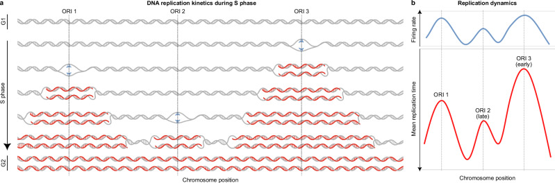
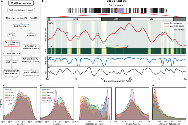
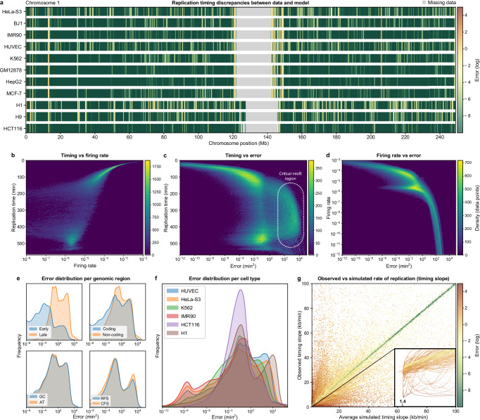
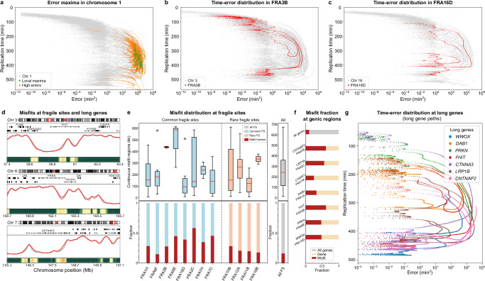
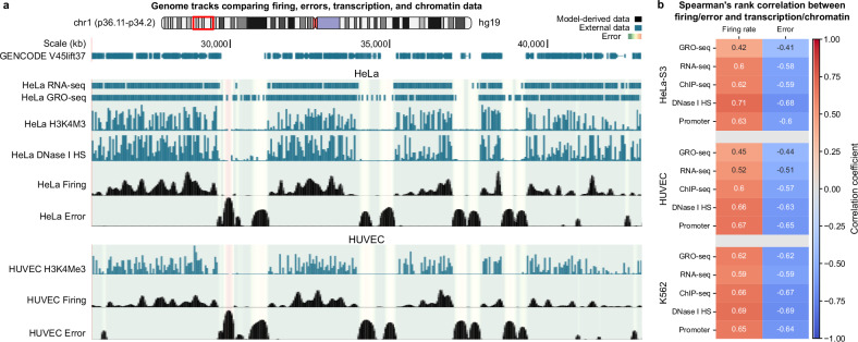
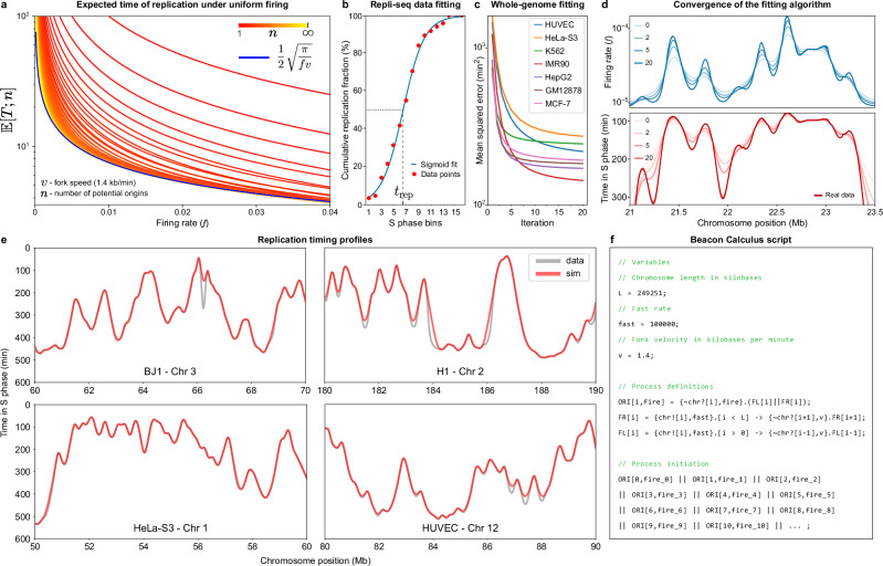
DNA replication in humans requires precise regulation to ensure accurate genome duplication and maintain genome integrity. A key indicator of this regulation is replication timing, which reflects the interplay between origin firing and fork dynamics. We present a high-resolution (1-kilobase) mathematical model that infers firing rate distributions from Repli-seq timing data across multiple cell lines, enabling a genome-wide comparison between predicted and observed replication. Notably, regions where the model and data diverge often overlap fragile sites and long genes, highlighting the influence of genomic architecture on replication dynamics. Conversely, regions of strong concordance are associated with open chromatin and active promoters, where elevated firing rates facilitate timely fork progression and reduce replication stress. In this work, we provide a valuable framework for exploring the structural interplay between replication timing, transcription, and chromatin organisation, offering insights into the mechanisms underlying replication stress and its implications for genome stability and disease.


Conflict of interest statement

Competing interests: The authors declare no competing interests.

Figures

Fig. 1
Fig. 1. A kinetic model of DNA replication.
a Replication initiates at specific origins that are licensed by the end of G1 phase. During S phase, replication forks progress bidirectionally from origins, passively replicating DNA until they merge with forks from adjacent origins or reach chromosome ends to complete replication and enter G2. In this example, three origins (ORIs 1, 2, and 3) fire at different times, with nascent DNA strands shown in red. At the end of replication, two identical copies of the original template are formed. b Illustration of the expected inverse but non-trivial correlation between firing rates (top) and replication timing (bottom, with an inverted y-axis). In a model where the firing time of each origin is an exponentially distributed random variable, the firing rate is the parameter of this distribution and tends to decrease as replication timing increases, indicating that regions with higher firing rates replicate earlier in S phase. Replication timing, measured by Repli-seq, shows the average replication time across a cell population, with peaks corresponding to potential origins. ORI 2 is in a late-replicating region, while ORI 3 replicates earlier, as indicated by their relative positions on the timing curve. Adapted from Hulke et al..
Fig. 2
Fig. 2. Predicting genome-wide features of replication.
a Overview of the main model and analysis. Starting with Repli-seq timing data, origin firing rates are fitted through Eqs. (1), (10), and (11). These rates generate expected timing profiles for comparison with experimental data to identify regions of timing misfits and fork stalling, which are analysed for correlations with other genomic processes. Simulations of replication features, such as fork directionality and inter-origin distances, validate the model against the literature. b Example of main modelling outputs from a region in HUVECs. Here we see the replication timing of both experimental and simulated data, and the magnitude of the misfit (error) for replication timing in a region where replication forks often stall; this leads to elevated errors that the model struggles to capture accurately. We also show the inferred origin firing rates and fork directionality, scaled between -1 (leftward) and +1 (rightward). We highlight three regions of interest: (1) A passively replicated site predominantly replicated by rightward-moving forks (RFD ~ 1); (2) A likely origin, characterised by a high firing rate and an RFD of 0; (3) A poorly fitted region between two origins with a low firing rate determined by the fitting algorithm with RFD of 0 (an equal likelihood of replication by leftward- and rightward-moving forks). c Kernel density estimate (KDE) of firing rate distributions across selected chromosomes in HUVECs. dg KDEs comparing genome-wide features—including firing rates, replication timing, fork directionality, and inter-origin distances—across different cell lines. All distributions align with experimental observations. Areas under curves are equal to 1, while y-axis values are omitted to emphasize relative shapes and distributions rather than absolute magnitudes.
Fig. 3
Fig. 3. Detecting discrepancies in replication timing determined experimentally and in simulations.
a Normalised error plots (red—high error, green—low error) highlighting deviations between simulated and experimental replication timings (chromosome 1 in various human cell lines). Grey areas: missing or unavailable data. bd Density scatter plots illustrating key relationships in H1 cells (averages of 500 simulations). Pairwise combinations of three variables are shown: replication time, firing rate, and error. In b, the inverse correlation between replication timing and firing rate is evident, with greater variability in firing rates late in S phase. c shows the relationship between replication timing and error, revealing that high errors are distributed throughout S phase (dotted oval). d illustrates the branching relationship between firing rate and error. e Error distributions in HUVEC cells, grouped by replication timing (early vs. late), genic vs. intergenic regions, GC vs. AT content, and classification of fragile sites (common vs. rare, CFS vs. RFS). f Genome-wide error profiles in different cells. g Scatter plot comparing average simulated timing slope, indicative of the progress of replication over time, against observed data, colour-coded by associated error. The zoomed-in region at [1.2, 2] × [0, 2] kb/min highlights the 1.4 kb/min bound on the simulated slope. Each dot represents a simulated-observed data pair, with the strand-like continuity arising from the high resolution of our 1 kb model, where proximity between adjacent pairs reflects the minimal positional shifts captured at this scale.
Fig. 4
Fig. 4. Timing errors in fragile sites and long genes.
a Replication timing vs. error on chromosome 1 in H1, highlighting regions with local maxima in error and neighbouring high-error zones (within a 300 kb radius). The threshold for identifying local maxima in errors is set at 102.8 (min2). Each dot represents an error-timing data pair, with the strand-like continuity arising from the high-resolution of our 1 kb model. b, c Genome-wide scatter plots displaying replication timing vs. error, with specific focus on common fragile sites FRA3B and FRA16D, revealing a continuous error path in mid-to-late replication, near the FHIT and WWOX genes, respectively. d Examples of misfit regions detected by the model across three different chromosomes (3, 6, and 7). Each panel shows the chromosome ideogram, gene locations, and a comparison between the observed data (grey) and model predictions (red), as well the associated error. Notably, misfit regions overlap with long genes such as FHIT (Chr 3), PRKN (Chr 6), and CNTNAP2 (Chr 7). e Misfit distribution for common (blue) and rare (pink) fragile sites, compared with the total fragile site misfit fraction (grey). Top: length (in Mb) of continuous misfit regions. Box plots show the median (middle line), 25th–75th percentiles (box), whiskers up to 1.5 times the interquartile range, and outliers (open circles). In total, 1262 continuous misfit regions across all fragile sites were analysed to illustrate global trends. Bottom: normalised misfit fraction at different sites. f Misfit fraction analysis of whole-genome genic regions, and at the largest genes within fragile sites (normalised). g Scatter plot of replication timing vs. error trajectories for long genes, highlighting error accumulations based on gene size and location within fragile sites.
Fig. 5
Fig. 5. Replication timing discrepancies and firing rate profiles correlate with transcriptional and chromatin data.
a Snapshot from the UCSC Genome Browser showing a detailed view of chromosome 1 (p36.11-p34.2) in HUVEC and HeLa (hg19). Various tracks compare transcriptional and chromatin data to misfit magnitude (error) and firing rate profiles obtained from our model (log-scale). Tracks include RNA-seq (marking mature mRNA levels), GRO-seq (nascent RNA), ChIP-seq for H3K4Me3 (promoters), and DNase I hypersensitivity (open chromatin). The error for each line is represented as a translucent heat map across tracks, with colours ranging from green (good fit) to yellow/red (poor fit). b Heatmap displaying the Spearman correlation coefficients between origin firing rates and fit errors with transcriptional and chromatin features for HeLa, HUVEC, and K562. All tests (two-sided) returned p-value < 10−15.
Fig. 6
Fig. 6. Fitting the model.
a Replication asymptotics under uniform firing: logarithmic plot of the expected replication time, E[T;n], as a function of the firing rate, f, and the number of potential origins, n (spaced at 1 kb intervals), for 1 ≤ n < , with v = 1.4 kb/min. As n → , E[T;n] approximates an inverse power law (blue). b Curve fitting for cumulative replication in S phase. Red markers depict example data points from a high resolution Repli-seq heatmap that shows the cumulative percentage of completed replication across 16 S phase bins. The blue line is the curve fitted to this data, while the dashed grey line indicates the median replication time, trep (the instant in S phase when 50% of replication is achieved across the cell population). c Whole-genome mean squared error between simulated timing profiles and real data for 7 cell lines, in min2. Fitting each line took ~3 min on a HPC platform (one CPU). d Progression of the fitting algorithm over 20 iterations for chromosome 2 in the BJ line on firing rates (above), with iteration 0 corresponding to the initial inverse power law estimate, given by Eq. (7), and the corresponding timing profile (below). e Observed (Repli-seq) timing against the simulated profiles for different lines and genomic regions. f Model written in the Beacon Calculus process algebra. Origin firing processes take their location, i (1-kb resolution), and firing rate fire, as parameters, triggering two replication fork processes, FL (left-moving) and FR (right-moving). Replication terminates when all locations have been replicated. The simulation begins by invoking the ORI processes, where fire_i corresponds to the firing rate values for each origin i, as determined by fitting Eq. (1).

Similar articles

References

    1. Gefter, M. L. DNA replication. Annu. Rev. Biochem.44, 45–78 (1975). - PubMed
    1. Leonard, A. C. & Méchali, M. DNA replication origins. Cold Spring Harb. Perspect. Biol.5, a010116 (2013). - PMC - PubMed
    1. Waga, S. & Stillman, B. The DNA replication fork in eukaryotic cells. Annu. Rev. Biochem.67, 721–751 (1998). - PubMed
    1. Mirkin, E. V. & Mirkin, S. M. Replication fork stalling at natural impediments. Microbiol. Mol. Biol. Rev.71, 13–35 (2007). - PMC - PubMed
    1. Rhind, N. & Gilbert, D. M. DNA replication timing. Cold Spring Harb. Perspect. Biol.5, a010132 (2013). - PMC - PubMed

LinkOut - more resources