. 2025 May 19;15(5):e71226.
doi: 10.1002/ece3.71226. eCollection 2025 May.

Growing Season Lengthens in a North American Deciduous Woody Community From 1993 to 2021

Affiliations

Growing Season Lengthens in a North American Deciduous Woody Community From 1993 to 2021

Carol K Augspurger et al. Ecol Evol. .

Abstract

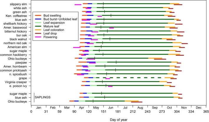
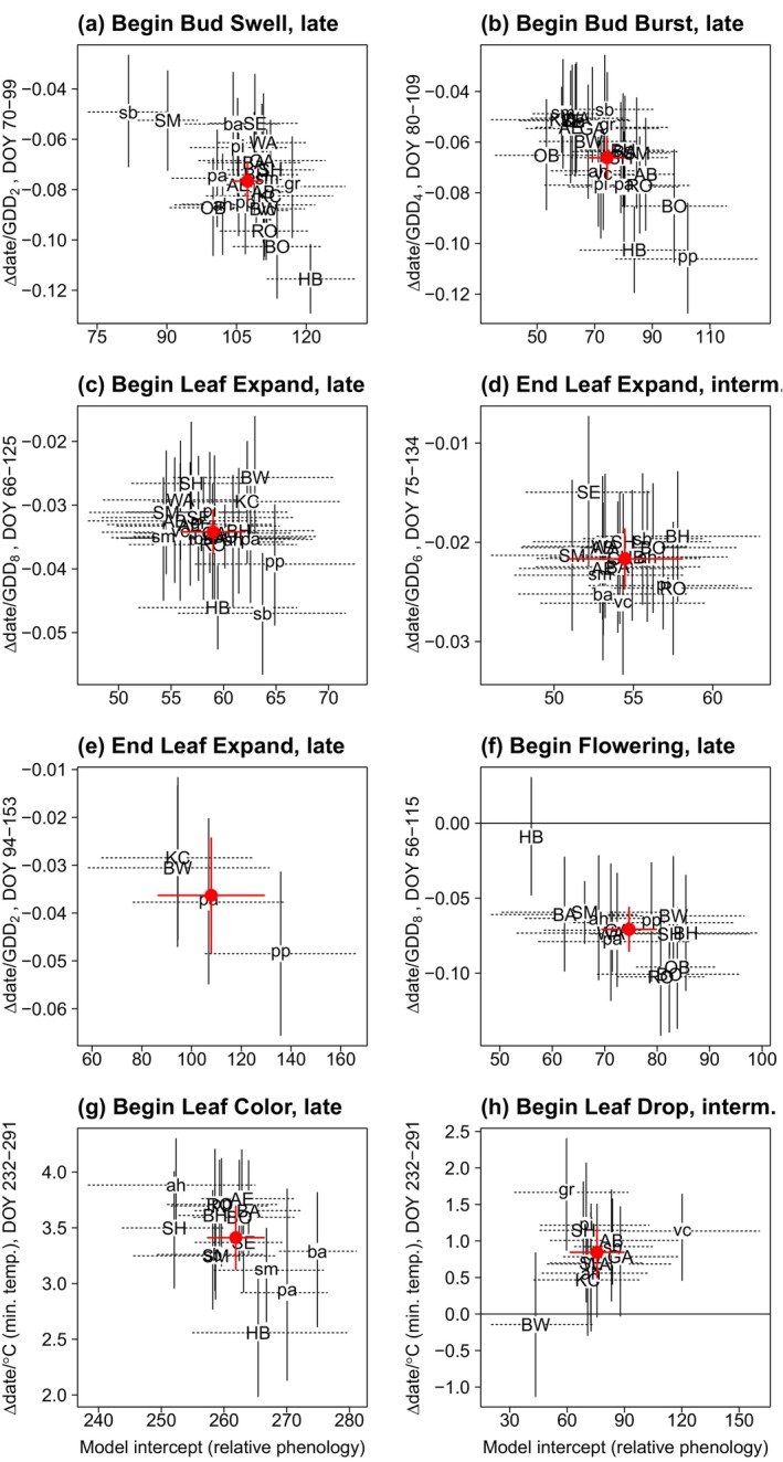
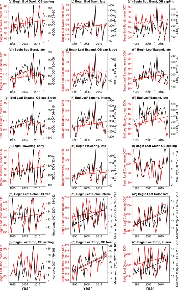
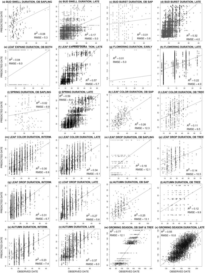
Observations of both spring and autumn phenological events were made annually over 29 years (1993-2021) for 22 taxa of multiple growth forms in a mature deciduous forest remnant near Urbana, Illinois, USA. Temporal trends in event dates, trends in stage durations, and associations with weather variables were analyzed with linear mixed-effect models. Species were grouped together in analyses based on seasonality.Spring event dates for most species advanced from 1.2 to 3.0 days/decade, while durations of spring stages shortened from 0.3 to 0.6 days/decade.Autumn event dates for most species delayed from 1.2 to 3.3 days/decade, while durations of autumn stages lengthened from 0.8 to 3.8 days/decade.Overall, the duration of the growing season lengthened for 88% of species (mean of 4.7 days/decade), with greater delays in autumn phenology for canopy trees and greater advances in spring phenology for other woody life forms.In spring, warmer mean daily temperatures were associated with advances in dates of phenological events. In autumn, minimum daily temperature in the preceding month(s) had the highest predictive power for seasonal groups, except those with Aesculus glabra.In autumn, most species had both a delay in phenology and a strong weather predictor, minimum daily temperature in September, that increased significantly through 29 years. In spring, some concordance between advancing event dates and warming spring temperatures were evident after removing data from 2018 to 2021 with especially high variability in spring temperatures.This study supports the hypothesis that climate change is showing a pronounced association with a delay in autumn leaf coloration, and less so an advance of spring leaf expansion. These changes can affect ecological processes, including plant productivity and carbon uptake/storage, assembly of communities, interactions between trophic levels, and species ranges and invasions.

Keywords: autumn phenology; climate change; long‐term; phenology; spring phenology.


Conflict of interest statement

The authors declare no conflicts of interest.

Figures

FIGURE 1
FIGURE 1
Annual phenology of each study species from 1993 to 2021 in Trelease Woods, Illinois, USA. See Appendix A: Table A5 for species nomenclature. Values plotted are mean dates per phenological event across all years; within a given year, the value for an event was calculated as the mean date across individuals of a given species. Species are ordered by mean date of beginning of bud swell, first by canopy tree species, then by treelets, shrubs, and vines, and finally by saplings of three canopy tree species. The vertical line indicates the date of full leaf maturity; the dark green line to the left of the vertical line indicates the period during which the fully expanded leaf is maturing. The dotted dark green line for grape indicates opportunistic growth of the vine for irregular periods of time. Not all species were used in analysis of a given event (see Appendix A: Table A5).
FIGURE 2
FIGURE 2
Change per year in 14 event dates versus relative phenology, for each species. Species are separated into seasonal groups for each event. Negative values on the y‐axis indicate earlier dates (advances), positive values later dates (delays). Values on the x‐axis indicate relative phenology (random species intercepts), where lesser values indicate species with earlier phenology. Solid vertical lines and dashed horizontal lines give the 95% bootstrap CI. Change in days represents the coefficient (random species slope, b) from linear mixed‐effects models, while the model intercept is the random species intercept from those models, as in the equation date = b(year) + intercept, where the year 1993 is set to year = 0. Two letters refer to abbreviation of the common name (see Appendix A: Table A5). The large red dot is the coefficient of the same variables from the seasonal group‐level analysis (±2 SE; red vertical and horizontal lines; Appendix C: Tables C2a and C2b). For red dots with no vertical SE, the top model did not include year as a fixed effect, that is, the event date did not change through time.
FIGURE 3
FIGURE 3
Change per year in 12 stage durations versus relative phenology, for each species. Negative values on the y‐axis indicate shortening durations, while positive values indicate lengthening durations. Values on the x‐axis indicate relative phenology (random species intercepts), where lesser values indicate species with shorter durations. See Figure 2 legend and Appendix C: Table C2c for additional details.
FIGURE 4
FIGURE 4
For each species of (a) canopy trees and (b) non‐canopy trees (* = sapling of canopy tree) over 1993–2021, a comparison of the number of days of change per year in spring (Begin Leaf Expansion; left dot) versus autumn (Begin Leaf Coloration; right dot) as a function of mean day of year of the event. Advances have negative values and delays have positive values. A black circle indicates the season that resulted in greater change in length of Growing Season; steeper slopes indicate a greater change in its length. Values were derived from each species' random slope coefficient for each event in the top mixed‐effects model (Appendix C: Tables C4a, C4b, C3c, C3d).
FIGURE 5
FIGURE 5
Change in date of seven events per weather variable unit (thermal sensitivity) versus relative phenology, for each species. Species are separated into seasonal groups for each event. Solid vertical lines and dashed horizontal lines give the 95% bootstrap CI. The relationship for a given event was included in this figure only if there was a weather variable that performed consistently as a predictor (Appendix C: Table C6) and random‐species slopes were included for that variable (Appendix C: Tables C4a, C4b, C10a, and C10b). Change in date per weather variable unit is the random‐species slope for the top model describing the relationship (Appendix C: Tables C7a and C7b), while relative phenology date is the random‐species intercept from the model. Smaller model intercept (x‐axis) values correspond with earlier phenological events. Letters refer to species' common names (see Appendix A: Table A5 for species and abbreviations). The large red dots represent the overall model coefficients for all species in the seasonal group‐level analyses (±2 SE; red vertical and horizontal lines; Appendix C: Table C6). All values in this figure represent the results of analyses based on untransformed (i.e., not standardized) values.
FIGURE 6
FIGURE 6
Inter‐annual variability in mean date of 18 phenological event‐by‐season combinations (red values) and the strongest weather model predictor for each (black values) from 1993 to 2021. Note that “OB” refers to Ohio buckeye, “Mean temp.” refers to mean daily mean temperature, and “Minimum temp.” refers to mean daily minimum temperature. When multiple weather variables were in the top five models (Appendix C: Tables C5a and C5b), the variable chosen had the highest absolute t‐value in the top model (Appendix C: Table C6). An inverted scale for the event date (left Y‐axis) was used for events that were negatively correlated with the weather predictor (all panels except L, N, O, and R). For weather variables, solid black regression lines represent the least‐squares regression through time when a significant trend was present (p < 0.05; Appendix C: Tables C9a and C9b), while no line indicates a non‐significant trend. For phenological events, solid red regression lines were created from the parameters in the change‐through‐time mixed‐effects model (Appendix C: Tables C1a and C1b); panels where red regression lines are absent represent cases in which year was not included in the top model (Appendix C: Tables C1a and C1b). Dashed lines show significant temporal trends from 1993 to 2017 for the weather variable (dashed black line) and event date (dashed red line) in cases with nonsignificant trends through 2021. A black asterisk (*) indicates that both phenology and weather variables have significant trends from 1993 to 2021, indicating support for the hypothesis that phenology has shifted with climate change. A red asterisk indicates that both phenology and weather variables had significant trends from 1993 to 2017, but not when including the last four years of data collection (driven by an extreme spring in 2018). End Leaf Drop (Late) is not presented because it had no weather variable in four of the top five models.
FIGURE D1
FIGURE D1
Validation of top temporal models for five spring phenological events of woody species at Trelease Woods (1993–2021) (A–K). Species are separated into two to three seasonal groups for each phenological event, yielding 11 event–season combinations. R 2 values indicate the coefficients of determination for observed values and the predicted values from the model. We used 10‐fold cross‐validation to evaluate model fit, and report the root‐mean‐square error (RMSE). Trend lines represent the least‐squares regression of the predicted and observed values.
FIGURE D2
FIGURE D2
Validation of top temporal models for four autumn phenological events of woody species at Trelease Woods (1993–2021) (A–O). Species are separated into 2–4 seasonal groups for each phenological event, yielding 16 event‐season combinations. R 2 values indicate the coefficients of determination for observed values and the predicted values from the model. We used 10‐fold cross‐validation to evaluate model fit, and report the root‐mean‐square error (RMSE). Trend lines represent the least‐squares regression of the predicted and observed values.
FIGURE D3
FIGURE D3
Validation of top temporal models for nine durations of phenological stages of woody species at Trelease Woods (1993–2021) (A–X). Species are separated into 2–4 seasonal groups for each stage, yielding 24 stage–season combinations. R 2 values indicate the coefficients of determination for observed values and the predicted values from the model. We used 10‐fold cross‐validation to evaluate model fit, and report the root‐mean‐square error (RMSE). Trend lines represent the least‐squares regression of the predicted and observed values.
FIGURE D4
FIGURE D4
Validation of top weather models predicting seven phenological events of woody species at Trelease Woods (1993–2021) (A–S). Species are separated into 2–4 seasonal groups for each phenological event, resulting in 19 event–season combinations. R 2 values indicate the coefficients of determination for observed values and the predicted values from the model. We used 10‐fold cross‐validation to evaluate model fit, and report the root‐mean‐square error (RMSE). Trend lines represent the least‐squares regression of the predicted and observed values.

Similar articles

References

    1. Archetti, M. , Richardson A. D., O'Keefe J., and Delpierre N.. 2013. “Predicting Climate Change Impacts on the Amount and Duration of Autumn Colors in a New England Forest.” PLoS One 8: e57373. - PMC - PubMed
    1. Augspurger, C. K. 2004. “Development Versus Environmental Control of Early Leaf Phenology in Juvenile Ohio Buckeye ( Aesculus glabra ).” Canadian Journal of Botany 82: 31–36.
    1. Augspurger, C. K. 2008. “Early Spring Leaf out Enhances Growth and Survival of Saplings in a Temperate Deciduous Forest.” Oecologia 156: 281–286. - PubMed
    1. Augspurger, C. K. 2009. “Spring 2007 Warmth and Frost: Phenology, Damage and Refoliation in a Temperate Deciduous Forest.” Functional Ecology 23: 1031–1039.
    1. Augspurger, C. K. 2011. “Frost Damage and Its Cascading Negative Effects on Aesculus glabra .” Plant Ecology 212: 1193–1203.

LinkOut - more resources