Comparison of Long-Term Air Pollution Exposure from Mobile and Routine Monitoring, Low-Cost Sensors, and Dispersion Models

Abstract

Introduction: Assessment of long-term exposure to outdoor air pollution remains a major challenge for epidemiological studies. One of these challenges is characterizing fine-scale spatial variation of the ambient concentrations of key traffic-related air pollutants - including ultrafine particles (UFPs), black carbon (BC), and nitrogen dioxide (NO₂). Epidemiological studies have used widely different approaches to address these challenges, including empirical land use regression (LUR) models based on fixed-site routine or targeted monitoring, low-cost sensor networks, mobile monitoring, and deterministic dispersion models. Little information is available about the relative performance of these different approaches for assessing long-term exposure to traffic-related air pollution. Different methods may result in heterogeneity in health effect estimates from epidemiological studies applying different exposure-assessment approaches.

The Specific Aims of the study.

1. Develop long-term ambient air pollution exposure estimates for selected epidemiological studies based on low-cost sensors, mobile and fixed-site monitoring, and deterministic dispersion modeling.

2. Compare different exposure assessment methods in terms of their ability to predict spatial variation of long-term average concentrations using external validation data.

3. Compare different exposure assessment methods in terms of air pollution effect estimates in selected epidemiological studies.

We assessed UFPs, NO₂, BC, and particulate matter ≤2.5 μm in aerodynamic diameter (PM_2.5).

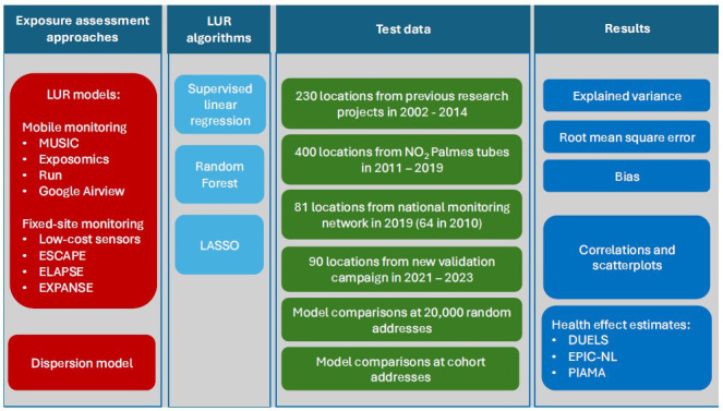
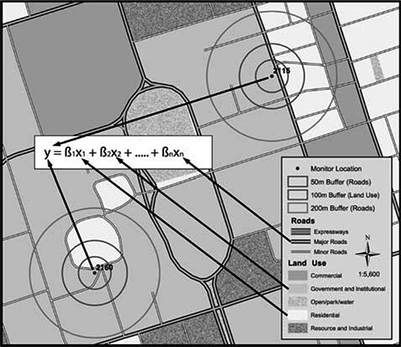
Methods: We evaluated annual average air pollution concentrations across the Netherlands using a suite of different exposure models, which differed in modeling approach (empirical LUR, deterministic dispersion models) and monitoring data used (low-cost sensors, mobile monitoring, nationwide and Europewide routine monitoring, and study-specific targeted monitoring). For empirical models, we tested three model development algorithms: supervised linear regression (SLR), Random Forest, and least absolute shrinkage and selection operator (LASSO). The predictions of the models were compared at 20,000 addresses across the Netherlands. The performance was also tested on external validation data, which were obtained from a new campaign (2021-2023) and existing data from different years, allowing assessment of how well recent models predict past air pollution exposure. Epidemiological analyses in three cohort studies were conducted to compare health effect estimates of the different exposure models. We assessed associations of air pollution in a national administrative cohort with natural-cause and cause-specific mortality, in a cohort study that had detailed lifestyle data with natural-cause mortality and incidence of stroke and coronary events, and in a mature birth cohort with lung function and asthma incidence.

Results: Exposure predictions at residential sites from the dispersion model and the Europewide hybrid LUR models were available for multiple years in the period 2010-2019. For these models, exposure predictions of different years in the period 2010-2019 were highly correlated for BC, NO₂, and PM_2.5 (Correlation coefficient R > 0.9). Consistently, the year of the exposure model did not affect the presence of an association with mortality and morbidity. Small differences in hazard ratios (HR) were related to exposure contrast for different years. The HR for the association of NO₂ with natural-cause mortality was 1.026 (95% confidence interval [CI]: 1.022-1.031) for the 2010 exposure estimate and 1.030 (1.024-1.035) for the 2019 exposure estimate of the Europewide LUR model, expressed per 10 µg/m³.

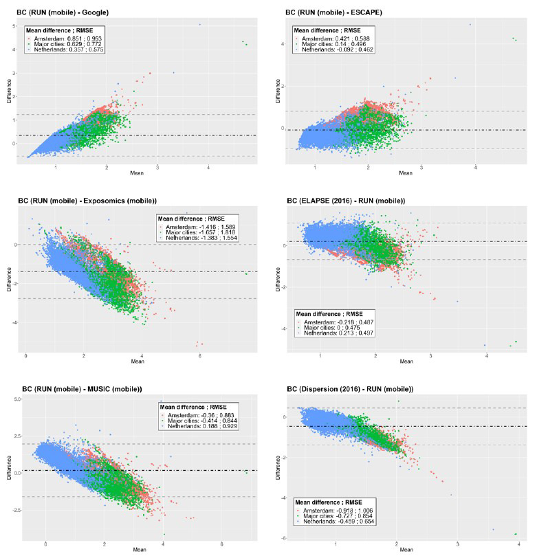
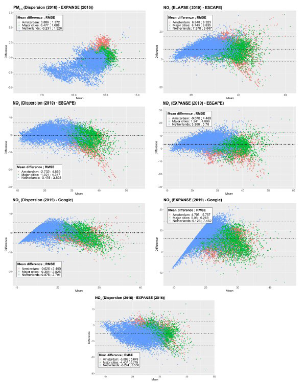
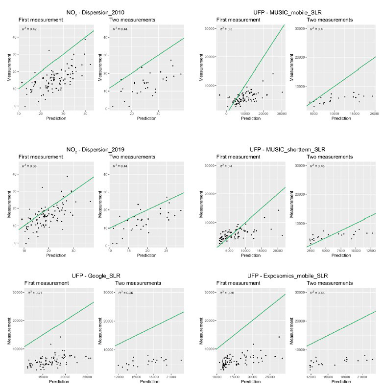
The exposure models generally resulted in highly to moderately correlated exposure predictions at residential sites across the Netherlands (R > 0.7 for BC, NO₂, and UFPs; R > 0.5 for PM_2.5). The predicted level of exposure and exposure contrast could differ substantially between models and algorithms within models; for example, the interquartile range (IQR) for BC for each of the various models at the 20,000 residential locations ranged between 0.1 and 2.2 µg/m³. Mobile monitoring studies generally resulted in modestly higher BC concentrations and exposure contrasts compared to other exposure models. Small differences were found between the different models in explaining the spatial variation of air pollution concentrations at the new and existing validation sites. Models explained historical exposure patterns at external sites covering more than 10 years moderately well, especially for BC (R > 0.7) and NO₂ (R > 0.7), and moderately so for UFPs (R > 0.5). Most models predicted the small concentration contrasts of PM_2.5 relatively poorly.

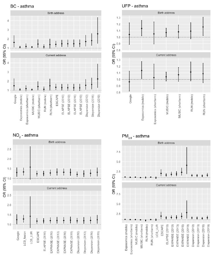
Consistent with the high correlation of the different exposure models, the application of these models generally resulted in similar conclusions on the presence of associations with natural-cause, respiratory, and lung cancer mortality in the large nationwide cohort, and with asthma incidence and lung function in the birth cohort. However, the effect estimates differed substantially; for example, the HR for natural-cause mortality in the nationwide administrative cohort for a 1 µg/m³ increase in BC ranged from 1.01 (95% CI: 0.99-1.02) to 1.09 (1.07-1.10). For the outcomes with small effect estimates and the smaller cohort studies, differences in conclusions related to the exposure assessment method were more distinct.

Differences in exposure assessment may contribute substantially to the observed heterogeneity of effect estimates in systematic reviews of epidemiological studies. High heterogeneity was indicated by the commonly used heterogeneity measure I², where the value was above 80% for a meta-analysis of the different effect estimates for natural-cause mortality in the nationwide cohort.

Validation of long-term exposure models for the nonroutinely monitored pollutants BC and especially UFPs was challenging, despite generally successful monitoring. The new external validation monitoring campaign resulted in rather unstable estimates of the long-term average spatial contrast, both across sites and where affected by temporal variation, especially for BC and PM_2.5.

No consistent differences were found in the model performance of SLR, Random Forest, and LASSO, both in internal cross-validation of model building and on external validation sites not used in model building. Exposure predictions from the three algorithms were generally highly correlated and resulted in similar associations with health. However, for individual models, occasionally large differences were found in exposure contrast, validation statistics, and associations with mortality and morbidity outcomes.

There was little benefit in using low-cost sensors for NO₂ and PM_2.5. The addition of low-cost sensor data did not improve NO₂ estimates in models that combined dispersion model estimates and data from the national monitoring network data.

Conclusions: The main conclusions of the project.

• Exposure predictions of BC, NO₂, and PM_2.5 for different years between 2010-2019 were highly correlated, documenting stable spatial contrast patterns. Consistently, the year of the exposure model did not affect the presence of an association with mortality and morbidity outcomes.

• Models explained historical exposure patterns at external sites covering more than 10 years moderately well, especially for BC.

• Different exposure models generally resulted in highly to moderately correlated exposure predictions. The predicted level of exposure and exposure contrast could differ substantially between models. Small differences were found between the different models in explaining spatial variation at validation sites.

• Application of different exposure models resulted in similar conclusions about the presence of associations with health outcomes, but effect estimates differed substantially in magnitude between individual exposure models. No consistent differences in effect estimates were found between groups of mobile, dispersion, and fixed-site LUR models.

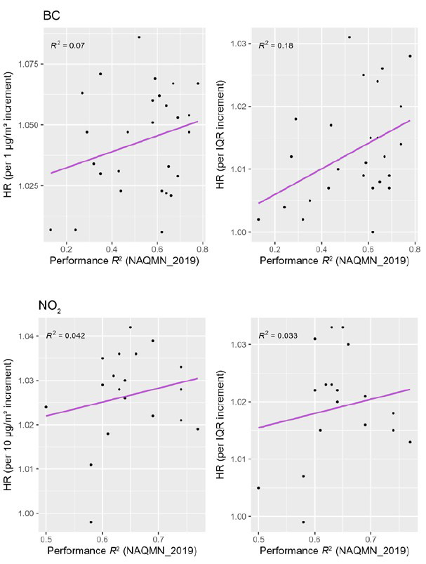
• Differences in exposure models may therefore contribute substantially to the observed heterogeneity of effect estimates in systematic reviews of epidemiological studies. Factors that explained some of the heterogeneity of effect estimates included the performance of the model at external validation sites and the predicted exposure contrast.

• Exposure predictions from the three algorithms were generally highly correlated and resulted in similar associations with health. No consistent differences were found in their model performances.

Statement Figure 1.

Schematic overview of the study design. LUR = land use regression

Figure 1.

Design of the project comparing the various exposure-assessment models. Pollutants assessed are UFPs, NO₂, BC, and PM_2.5. For the empirical models, three algorithms were applied. Table 1 explains the models.

Figure 2.

Distribution of all hourly measurements of PM_2.5 during both field campaigns for the sensors (blue) and stations (red) of the NAQMN.

Figure 3.

Validation metrics for the at-distance night-time calibration at participant locations, validated at NAQMN station Kardinaal de Jongweg. Left figure: Pearson correlation. Middle figure: Root Mean Square Error (μg/m³). Right figure: Average concentration (μg/m³) including the reference concentration in black. The x-axis shows the distance (m) to the reference station that was used to recalibrate. To estimate the quality of a calibration that does not use the raw NO₂ sensor signal as a predictor, the green circles indicate a prediction (linear regression) using only T and O₃ as predictor variables. The blue triangles show the improvement in validation statistics for the NO₂ sensor calibration which uses the raw NO₂-sensor signal, T, and O₃ as predictor variables.

Figure 4.

Map of the average PM_2.5 concentrations (μg/m³), for 10/2/2021–03/31/2022, based on all sensors (dots) and all their nearest NAQMN station average (squared dots).

Figure 5.

Weekly (upper) and daily (bottom) pattern of NO₂ concentrations for 10/2/2021–03/31/2022, based on all sensors (grey lines) and their average (blue line). The shaded area resembles the ± 2 times standard deviation.

Figure 6.

Weekly (upper) and daily (bottom) pattern of PM_2.5 concentrations for 10/2/2021–03/31/2022, based on all sensors (grey lines) and their average (blue line). The shaded area resembles the ± 2 times standard deviation.

Figure 7.

Weekly average NO₂ concentration of several model variants compared with concentrations (μg/m³) from the new external validation campaign (section 5.5). Model variants: Standard RIVM model with countrywide fusion of reference measurements (Mean_All_0), countrywide fusion of model with reference and sensor measurements (Mean_All_0.5), regional (North–South) fusion of model with reference and sensor measurements (mean_Region_NS_0.5), and regional (West–East) fusion of model with reference and sensor measurements (mean_Region_WE_0.5). The green line is the 1:1 line.

Figure 8.

Correlation of exposure estimates of multiple years at the 20,000 residential sites from dispersion modeling for BC, NO₂, and PM_2.5. The green line is the 1:1 line. The scale of the y-axis of the top-left graph refers to the density plot (density times concentration difference of an interval is the probability of that interval), the remaining y-axes to absolute concentrations (in μg/m³).

Figure 9.

Correlation of exposure estimates from different models at 20,000 residential sites across the Netherlands for BC, NO₂, UFPs, and PM_2.5. The green line is the 1:1 line. The scale of the y-axis of the top-left graph refers to the density plot (density times concentration difference of an interval is the probability of that interval); the remaining y-axes to absolute concentrations (in μg/m³, except UFPs in p/cm³).

Figure 10.

Bland-Altman plots of predicted annual average concentrations of exposure models at residential address across the Netherlands (blue), green (major cities), and Amsterdam (orange) for BC, PM_2.5, and NO₂ (μg/m³). Lines represent mean difference and 95% confidence intervals for the Netherlands.

Figure 10.

Bland-Altman plots of predicted annual average concentrations of exposure models at residential address across the Netherlands (blue), green (major cities), and Amsterdam (orange) for BC, PM_2.5, and NO₂ (μg/m³). Lines represent mean difference and 95% confidence intervals for the Netherlands.

Figure 10.

Bland-Altman plots of predicted annual average concentrations of exposure models at residential address across the Netherlands (blue), green (major cities), and Amsterdam (orange) for BC, PM_2.5, and NO₂ (μg/m³). Lines represent mean difference and 95% confidence intervals for the Netherlands.

Figure 11.

Distribution of average measurements at 90 new external validation sites, adjusted for temporal variation, stratified by site type. RB = regional background, T = traffic, UB = urban background.

Figure 12.

Comparison of exposure predictions from different models with weekly average measurements adjusted for temporal variation at the new external validation sites for NO₂ and UFPs. SLR models only, selected years from dispersion and European models. NO₂ in μg/m³, UFPs in p/cm³. The green line is the 1:1 line.

Figure 12.

Comparison of exposure predictions from different models with weekly average measurements adjusted for temporal variation at the new external validation sites for NO₂ and UFPs. SLR models only, selected years from dispersion and European models. NO₂ in μg/m³, UFPs in p/cm³. The green line is the 1:1 line.

Figure 12.

Comparison of exposure predictions from different models with weekly average measurements adjusted for temporal variation at the new external validation sites for NO₂ and UFPs. SLR models only, selected years from dispersion and European models. NO₂ in μg/m³, UFPs in p/cm³. The green line is the 1:1 line.

Figure 13.

Scatterplots of comparison of exposure predictions with existing external validation data for BC, NO₂, UFPs, and PM_2.5. The green line is the 1:1 line. Pollutant concentrations are in p/cm³ for UFPs and in μg/m³ for all others. The first element of the title indicates the exposure prediction model (e.g., Google SLR model); the second is the validation data (see section 3.3.1).

Figure 13.

Scatterplots of comparison of exposure predictions with existing external validation data for BC, NO₂, UFPs, and PM_2.5. The green line is the 1:1 line. Pollutant concentrations are in p/cm³ for UFPs and in μg/m³ for all others. The first element of the title indicates the exposure prediction model (e.g., Google SLR model); the second is the validation data (see section 3.3.1).

Figure 13.

Scatterplots of comparison of exposure predictions with existing external validation data for BC, NO₂, UFPs, and PM_2.5. The green line is the 1:1 line. Pollutant concentrations are in p/cm³ for UFPs and in μg/m³ for all others. The first element of the title indicates the exposure prediction model (e.g., Google SLR model); the second is the validation data (see section 3.3.1).

Figure 13.

Scatterplots of comparison of exposure predictions with existing external validation data for BC, NO₂, UFPs, and PM_2.5. The green line is the 1:1 line. Pollutant concentrations are in p/cm³ for UFPs and in μg/m³ for all others. The first element of the title indicates the exposure prediction model (e.g., Google SLR model); the second is the validation data (see section 3.3.1).

Figure 13.

Scatterplots of comparison of exposure predictions with existing external validation data for BC, NO₂, UFPs, and PM_2.5. The green line is the 1:1 line. Pollutant concentrations are in p/cm³ for UFPs and in μg/m³ for all others. The first element of the title indicates the exposure prediction model (e.g., Google SLR model); the second is the validation data (see section 3.3.1).

Figure 14.

HR for the association of the four pollutants with natural mortality for different exposure models in the nationwide DUELS cohort, using the most adjusted model 3. HR expressed per 1-μg/m³ for BC, 10-μg/m³ for NO₂, 5,000-p/cm³ for UFPs, and 5-μg/m³ for PM_2.5. Covariates included were at the individual level age (time axis), sex (strata), standardized household income, region of origin (Dutch, Western, non-Western, Morocco, Turkey, Suriname, Antilles Netherlands), and marital status (married, widowed, divorced, single), and at area-level socioeconomic status variables at both the neighborhood and the regional (COROP) scale: mean income per income recipient, social assistance per 1,000 inhabitants, % low education, % non-Western immigrants, and unemployment per 1,000 inhabitants. IQR is shown in Appendix A table S1. Note scales differ per pollutant.

Figure 15.

Associations between BC and NO₂ with natural mortality of different exposure models in relation to the explained variance at NAQMN external validation sites in 2019. HR per 1- and 10-μg/m³ for BC and NO₂, and model-specific IQR. Models using the most adjusted model 3 (see Figure 14). IQR is shown in Appendix A Table S1. The purple line is the regression line. Note that scales differ per pollutant.

Figure 16.

Associations between air pollution exposure and asthma at age 1 to 20 years at the birth and current address, most adjusted model. OR expressed per 1-μg/m³ for BC, 10-μg/m³ for NO₂, 5,000-p/cm³ for UFPs, and 5-μg/m³ for PM_2.5. Adjusted for sex, maternal and paternal asthma, hay fever, native nationality, parental education, breastfeeding, older siblings, day-care attendance, maternal smoking during pregnancy, parental smoking at home, mold or dampness at home, pets, use of gas for cooking, and active smoking (from age 14). Note scales differ per pollutant.

Figure 17.

Associations between air pollution exposure and lung function (FVC and FEV1) at age 16 at the current address, most adjusted model. Expressed as percentage difference for fixed increments: 1-μg/m³ for BC, 10-μg/m³ for NO₂, 5,000-p/cm³ for UFPs, and 5-μg/m³ for PM_2.5. Adjusted for sex, log-transformation of age, weight, and height, parental education, maternal atopy, paternal atopy, breastfeeding, respiratory infections in the last 3 weeks (before the medical examination), Dutch nationality, indoor tobacco smoke exposure in the home, maternal smoking in pregnancy, furry pets in the home, mold in the home, gas cooking, and average air pollution concentrations for the 7 days preceding the lung function measurement. Note that scales differ per pollutant.

Figure 18.

Associations between BC, NO₂, UFPs, and PM_2.5 with lung function of different exposure models in relation to the explained variance at NAQMN external validation sites in 2019. Most adjusted model. The purple line is the regression line.

Figure 18.

Associations between BC, NO₂, UFPs, and PM_2.5 with lung function of different exposure models in relation to the explained variance at NAQMN external validation sites in 2019. Most adjusted model. The purple line is the regression line.

Figure 19.

Associations between air pollution exposure and natural-cause mortality in EPIC-NL, most-adjusted model (N = 33,269). HR expressed per 1-μg/m³ for BC, 10-μg/m³ for NO₂, 5,000-p/cm³ for UFPs and 5-μg/m³ for PM_2.5. Covariates adjusted for include age (time axis), sex (strata), smoking status (never/former/current), smoking intensity (number of cigarettes/day), smoking duration (years of smoking), fruit and vegetable intake, alcohol consumption (low, medium, high), body mass index (BMI) (categories defined by WHO), educational level (low, medium, high), employment and occupational status (employed, unemployed, housekeeping, retired), marital status (single, married/with a partner, divorced, widowed) at the individual level, and mean income, ethnicity, and unemployment rate at the neighborhood level.

Commentary Figure 1.

Illustration of elements of a LUR model (Jerrett et al. 2005).

Commentary Figure 2.

Schematic overview of the study design.

References

-
- Apte JS, Messier KP, Gani S, Brauer M, Kirchstetter TW, Lunden MM, et al. . 2017. High-resolution air pollution mapping with Google Street View cars: exploiting big data. Environ Sci Technol 51:6999–7008, https://doi.org/10.1021/acs.est.7b00891. - PubMed
- van de Beek E, Kerckhoffs J, Hoek G, Sterk G, Meliefste K, Gehring U, et al. . 2021. Spatial and spatiotemporal variability of regional background ultrafine particle concentrations in the Netherlands. Environ Sci Technol 55:1067–1075, https://doi.org/10.1021/acs.est.0c06806. - PMC - PubMed
- Beelen R, Hoek G, Vienneau D, Eeftens M, Dimakopoulou K, Pedeli X, et al. . 2013. Development of NO2 and NOx land use regression models for estimating air pollution exposure in 36 study areas in Europe: the ESCAPE project. Atmos Environ 72:10–23, http://dx.doi.org/10.1016/j.atmosenv.2013.02.037.
- Blanco MN, Doubleday A, Austin E, Marshall JD, Seto E, Larson TV, et al. . 2023a. Design and evaluation of short-term monitoring campaigns for long-term air pollution exposure assessment. J Expo Sci Environ Epidemiol 33:465–473, https://doi.org/10.1038/s41370-022-00470-5. - PMC - PubMed
- Blanco MN, Bi J, Austin E, Larson TV, Marshall JD, Sheppard L. 2023b. Impact of mobile monitoring network design on air pollution exposure assessment models. Environ Sci Technol 57:440–450, https://doi.org/10.1021/acs.est.2c05338. - PMC - PubMed
Publication types
MeSH terms
Substances
LinkOut - more resources
Full Text Sources
Medical
Miscellaneous