Domesticated cannabinoid synthases amid a wild mosaic cannabis pangenome

Abstract

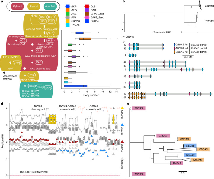
Cannabis sativa is a globally important seed oil, fibre and drug-producing plant species. However, a century of prohibition has severely restricted development of breeding and germplasm resources, leaving potential hemp-based nutritional and fibre applications unrealized. Here we present a cannabis pangenome, constructed with 181 new and 12 previously released genomes from a total of 144 biological samples including both male (XY) and female (XX) plants. We identified widespread regions of the cannabis pangenome that are surprisingly diverse for a single species, with high levels of genetic and structural variation, and propose a novel population structure and hybridization history. Across the ancient heteromorphic X and Y sex chromosomes, we observed a variable boundary at the sex-determining and pseudoautosomal regions as well as genes that exhibit male-biased expression, including genes encoding several key flowering regulators. Conversely, the cannabinoid synthase genes, which are responsible for producing cannabidiol acid and delta-9-tetrahydrocannabinolic acid, contained very low levels of diversity, despite being embedded within a variable region with multiple pseudogenized paralogues, structural variation and distinct transposable element arrangements. Additionally, we identified variants of acyl-lipid thioesterase genes that were associated with fatty acid chain length variation and the production of the rare cannabinoids, tetrahydrocannabivarin and cannabidivarin. We conclude that the C. sativa gene pool remains only partially characterized, the existence of wild relatives in Asia is likely and its potential as a crop species remains largely unrealized.

Fig. 1. Cannabis pangenome architecture uncovers at least five populations.

a, Genomic features of ten chromosome pairs in EH23. One million base pair rectangular windows extend from each haplotype at a width proportional to the absence of the CpG motif (high CpG content in centromeric and telomeric regions shown as constrictions). Each rectangular window is coloured by gene density, with warm colours indicating high gene density and cool colours indicating low gene density. Each haplotype pair is connected by polygons indicating structural arrangement, with grey for syntenic regions and orange connecting inversions. Rectangles along each haplotype indicate select loci, including 45S (26S, 5.8S and 18S) RNA arrays (firebrick red), 5S RNA arrays (black) and cannabinoid synthases (forest green). b, Summary of sex chromosomes based on haplotype-resolved XY assemblies^,. Phylogenetic analysis of XY homologues revealed variation in SDR-linked versus PAR-linked genes on the Y chromosome, as indicated by a clade of Y-linked homologues (Ya) versus a clade containing both X- and Y-linked homologues (Yb), respectively. Tip triangles indicate collapsed monophyletic clades of X or Y homologues. The X-specific region does not undergo recombination with the Y chromosome (although it undergoes recombination in XX females). c, Collector’s curve using shared gene orthogroup membership. d, Collector’s curve using shared 31-mers. e, Gene membership across all pangenome samples. f, Hierarchical clustering of Jaccard similarity scores based on 31-mers reveals a structure of at least 5 groups in the pangenome. Each drug-type group contains both MJ and HC hemp samples (Supplementary Table 1). Scale bar represents distance of maximum Jaccard dissimilarity. g, 31-mer-based multidimensional scaling plot of all pangenome assemblies (blue), Wild Tibet assembly (purple) and global diversity panel of short-read samples (green, ‘basal’ population from Asia; grey, other populations). Source data

Fig. 2. TEs shape the cannabis pangenome.

a, Percentage of genome covered by TEs, using 78 chromosome-level, haplotype-resolved genomes, grouped by population. The y axis shows the Gaussian kernel density estimation. b, Across the pangenome, the age distribution of fragmented TEs, with inset showing their distribution within the past 100,000 years. In the inset, the highest density occurs since 10 thousand years ago (ka). c, Age distribution of intact TEs, with inset showing distribution within the last 100,000 years. In the inset, the highest density occurs within 10 kya. d, Average solo:intact ratio for Ty1-LTR elements in 78 chromosome-level, haplotype-resolved genomes, grouped by chromosome. For all box plots, the green dashed line is the mean and the orange solid line is the median. The lower and upper edges of the box correspond to the lower and upper quartiles. The vertical lines (whiskers) extending from the box reflect the minimum and maximum values in the dataset. Each scatter point represents an individual genome. e, Average solo:intact ratio for Ty3-LTR elements. f, Average solo:intact ratio for Ty1-LTR elements in the sex chromosomes grouped according to boundary (PAR, X-specific region or SDR). g, Average solo:intact ratio for Ty3-LTR elements in the sex chromosomes grouped according to boundary (PAR, X-specific region or SDR). h, Genomic landscape plot for the AH3Mb Y chromosome, showing density of LTRs, methylation, CpG content and transcripts across the chromosome. i, Genomic landscape plot for the AH3Mb Y chromosome, showing the ratio of solo:intact Ty1-LTRs across the chromosome. j, Visualization of whole-genome alignments between the AH3Ma X and Y chromosomes. The bracketed region with high similarity is the PAR. k, Genomic landscape plot for the AH3Ma X chromosome, showing density of LTRs, methylation, CpG content and transcripts across the length of the chromosome. l, Genomic landscape plot for the AH3Ma X chromosome, showing the ratio of solo:intact Ty1-LTRs across the length of the chromosome. Source data

Fig. 3. Structural variants occur at different frequencies in populations and are non-randomly distributed across the genome.

a, Frequencies of inversions (inv), duplications (dup) and translocations (trans) by population. European hemp, Asian hemp and MJ populations differ significantly in average translocation and duplication counts, but not in inversions. Each box plot represents the median (centre line), two hinges (quartiles) and two whiskers (1.5× the interquartile range (IQR). b, Non-random genomic distribution of translocations (purple histograms), duplications (dark red bands) and inversions (mapped as length-scaled yellow bars on the right side of chromosomes, with each bar equal to one inversion). c, LD plot limited to 200-kb interactions, highlighting the general decay curves, with the X chromosome exhibiting a markedly reduced decay rate. Collectively, across the 78 haplotype-resolved, chromosome-scale assemblies, LD decay plots showed decay to half of the maximum r² value around 10 kb, which is similar to wild outcrossing soy and rice populations. d, LD decay plots extended to 800 kb. The increase in long-range (hundreds of kb to Mb) LD patterns found in certain SNP pairs further underscored the importance of using accurately phased genome assemblies and consideration of SVs for mapping and improvement efforts.

Fig. 4. The cannabinoid biosynthesis pathway is domesticated yet shows contrasting patterns of genetic diversity and synteny.

a, Cannabinoid biosynthesis pathway and gene copy numbers across the pangenome, per assembly. The left and right edges of the box plots correspond to the lower and upper quartiles, and the line in the box is the median. The horizontal lines that extend outward from the box (whiskers) reflect the minimum and maximum values in the dataset. Each scatter point represents an individual genome. AAE, acyl-activating enzyme; ACC, acetyl-CoA carboxylase; ACP, acyl carrier protein; CBCVA, cannabichromevarinic acid; CBDVA, cannabidivarinic acid; CBGVA, cannabigerovarinic acid; CoA, coenzyme; DH, dehydratase; DMAPP, dimethylallyl pyrophosphate; ENR, enoyl-ACP reductase; FASII, type II fatty acid synthase; GPPS, geranyl diphosphate synthase; IPP, isopentenyl diphosphate; KAS, β-ketoacyl-acyl carrier protein synthase; OAC, olivetolic acid cyclase; OLS, olivetolic acid synthase; THCVA, tetrahydrocannabivarin acid. b, Consensus maximum-likelihood phylogeny of aligned coding sequences from cannabinoid synthases, with the proportion of 100 bootstrap replicates shown on branches where values are greater than 0.75. Each branch tip represents a distinct cluster of synthases within greater than 99% identity of 859 total synthases from across all 193 pangenome samples. c, Summary of common cannabinoid synthase cassette arrangements, with the number of occurrences in the pangenome shown on the left. Full, full-length synthase gene models; partial, truncated lower-stringency synthase alignments that probably represent pseudogenes. d, Synthase cassettes exhibit variation in synteny, as seen in BUSCO anchored local alignment of chr. 7. Red triangle, THCAS cassettes; blue triangles, CBDAS cassettes; yellow triangle, CBCAS cassettes; grey triangles, low-stringency synthase matches (pseudogenes); grey and pink circles, BUSCOs. e, Maximum-likelihood tree of helitron DNA TE sequences flanking (2 kb upstream or downstream) cannabinoid synthase genes in the 78 haplotype-resolved, chromosome-scale assemblies. Source data

Fig. 5. ALT gene trans-duplication and diversification explains varin cannabinoid phenotype in cannabis.

a, PanKmer crossover analysis identifies the specific breakpoints on chr. 7 (vertical dashed lines) for the ALT gene haplotypes in relation to cannabinoid synthases. UFBb has one crossover at 5 Mb that breaks the linkage between HO40 (HO) THCAS and the varin haplotype ALT genes, whereas WCFBb has two crossovers, which result in an absence of the HO40 ALT alleles. b, ALT3 and ALT4 arrangements on chr. 7 of EH23a and EH23b. c, Protein-based neighbour-joining phylogeny, showing relationships between the three ALT3 orthogroup OG2876 members on chr. 7, including the three alternative splice variants (t1, t2 and t3) from the EH23a gene model, with the proportion of 100 bootstrap replicates shown on branches where values are greater than 0.50. d, Sequence tube map visualization of variation at ALT4 from the 16 haplotype graph pangenome incorporating the following colour-coded assemblies: 1, AH3Ma; 2, AH3Mb; 3, BCMa; 4, BCMb; 5, EH23a; 6, EH23b; 7, GRMa; 8, GRMb; 9, KCDv1a; 10, KCDv1b; 11, KOMPa; 12, KOMPb; 13, MM3v1a; 14, SAN2a; 15, SAN2b; 16, YMv2a. e, BKR 6-exon and 11-exon gene models and local nucleic acid alignment for EH23a and EH23b, with close up of the 2-bp deletion that truncates the 6-exon model. Green arrows, gene models; yellow arrows, coding sequences; red, blue, white and olive arrows, TEs. Green vertical bars represent per cent identity for the alignment. f, BKR protein-based neighbour-joining phylogeny from 772 pangenome gene models, with the proportion of 100 bootstrap replicates shown on branches where values are greater than 0.25.

Extended Data Fig. 1. PanKmer Jaccard similarity matrix of 193 Cannabis genomes.

PanKmer (PK) was used to estimate the relationship between the genomes in the cannabis pangenome. A large portion of the pangenome included elite cultivars, breeding trios and foundational Marijuana (MJ) lines originating from breeding programs spanning the 1970s to present (Supplementary Fig. 1; Supplementary Table 1). These samples represented chemotypes showing high expression of pentyl or propyl (varin) homologs of CBDA or THCA, and cannabinoid free (type V) plants. Flowering time variation was also captured with the inclusion of both short-day (SD) and DN phenotypes. The remaining cultivars came from the United States Department of Agriculture (USDA) Germplasm Resource Information Network (GRIN) and German federal genebank (IPK Gatersleben) repositories to ensure researchers will have access to plants for experimentation. These samples included European and Asian fiber and seed hemp, feral populations, North American marijuana (type I), hc yielding (CBDA or CBGA) hemp (type III and IV), male plants (XY; Fig. 1b) and monoecious plants (XX; Supplementary Table 1). Together, this comprehensive dataset provides a foundation for exploring cannabis genomic diversity, hybridization, and trait evolution. See Figshare for full resolution version.

Extended Data Fig. 2. The EH23 anchor genome sequencing strategy and resulting populations.

A) The F1 hybrid EH23 (ERBxHO40#23) was generated by crossing the type III (high CBDA), day neutral (DN), Early Resin Berry (ERB) with the type I (high THC), day sensitive (DS), HO40. Both ERB and HO40 were sequenced with PacBio CLR, while EH23 was sequenced with PacBio HiFi (CCS) and scaffolded with High-throughput Chromatin Conformation Capture (Hi-C). The F2 mapping population (288 individuals) was sequenced with Illumina short reads. The remaining pangenome samples from OCBD are summarized in (Supplementary Table 1) with a pedigree chart (Supplementary Fig. 1). B) Organization schematic for 193 genomes of the cannabis pangenome. Two methods were used to achieve haplotype-resolved, chromosome-scale genomes. The first, a streamlined method, employed Hi-C data for both phasing and scaffolding (Supplementary Table 1, Methods), generating 24 haploid genomes from 12 samples (Hifiasm_HiC). These served as scaffolding references for 42 genomes from 21 samples (Hifiasm_Trio_RagTag), resulting in trio-phased haploid assemblies. Together, these 78 genomes serve as the foundation for our pangenome analyses of transposable elements and structural variation. Additionally, we generated 20 haplotype-resolved contig-level assemblies (Hifiasm), along with 83 contig-level assemblies using older PacBio continuous long reads (CLR; 23 assemblies) and circular consensus sequencing (CCS; 60 assemblies) (Supplementary Table 1). C) Diagram of genomes used in different analyses for this study. For all assemblies we generated gene model annotations using both ab initio tools and RNA expression data, as well as TEs called using a RepeatModeler library (Supplementary Table 2, Methods).

Extended Data Fig. 3. F1 hybrid (ERBxHO40_23; EH23a and EH23b) between two phenotypically and genetically divergent parents clarifies features of the genome missed in other studies to-date.

A) Inheritance of alleles across the genome from the F2 population. The upper panel presents the frequency of each allele and the lower panel shows FIS or the deviation from our evolutionarily neutral expectation of heterozygosity. B) Haplotype specific expression for all tissue types from EH23, grouped by chromosome. Haplotype gene pairs were either syntenic or reciprocal best hits. Balanced and biased gene expression was assigned according to TPM difference. A difference threshold of 5 TPM was required for gene pairs to be assigned as biased, otherwise gene pairs were assigned as balanced (see also Supplemental Table 2 for counts by tissue type). C) LATE ELONGATED HYPOCOTYL (LHY) showed biased gene expression in EH23b foliage under 12 h of light (12/12 h). D) The copy of LHY with biased expression also belonged to an orthogroup with high entropy in different populations, with the largest difference in entropy separating feral and MJ. E) GO term enrichment of biased gene expression for all tissues in EH23a; and F) GO term enrichment of biased gene expression for all tissues in EH23b. See also Supplemental Note 2.

Extended Data Fig. 4. The cannabis pangenome and pangenes are high quality.

A) Benchmarking Universal Single-Copy Orthologs (BUSCO) for both the genome and gene predictions suggest that they are both high quality and complete. Gene models were predicted based on homology and expression data from different tissues, including flowers, leaves, and roots (Supplementary Table 2) with TSEBRA. We evaluated the quality of gene models with BUSCO, which were around 95% complete on average for all assembly types. The scaffolded genomes contained 35,000 genes on average, and in the contig genomes, the number of genes scaled with the presence of duplications detected by BUSCO (Fig. 1e). B) The number of genes predicted contrasted with the number of BUSCO duplicate genes suggesting that the CCS and CLR contig-based assemblies were retaining significant duplicated sequence due to uncollapsed haplotypes. These haplotypes were not removed to retain the level of variation for downstream analysis. C) Scatter plot of chromosome lengths on the x-axis compared with gene counts per chromosome on the y-axis across the nine autosomes and both sex chromosomes.

Extended Data Fig. 5. Cannabis centromere and telomere analysis shows higher order repeat structure.

A-B) The AceHigh3 (AH3M) chromosomal features of nine pairs of autosomes and one pair of sex chromosomes (X and Y). One million base pair rectangular windows extend outward from each pair of haplotypes at a width proportional to the absence of the CpG motif. Each rectangular window is colored by gene density with warm colors indicating high gene density and cool colors indicating low gene density. Each pair of haplotypes is connected by polygons indicating structural arrangement, with gray for syntenic regions and orange connecting inversions. Rectangles along each haplotype indicate select loci, including 45S (26S, 5.8S, 18S) rDNA arrays (firebrick red), 5S RNA arrays (black), 237 bp centromere repeat (blue), 370 bp CS-1 sub-telomeric repeat (pink) and cannabinoid synthases (forest green; CBCAS, CBDAS, THCAS, and OAC). Chromosomal plots for all 78 haplotype-resolved, chromosome-scale genomes show similar trends (see Ideos.pdf at https://doi.org/10.25452/figshare.plus.28405079.v1). C) The centromere arrays identified in the AH3M genome (as an exemplar for the pangenome) with Tandem Repeat Finder (TRF). Two high copy number arrays were identified with base repeats of 237 and 370 bp, along with their higher order repeats (HOR). The 237 bp array is sparsely found in the genome (blue, panel A), although usually proximal to the high “CpG” sites. The 370 bp repeat is the same sequence as the sub-telomeric repeat CS-1 and found on the ends of the chromosomes (pink, panel A). D) A subset of the genomes were sequenced on Oxford Nanopore Technologies to estimate the telomere length in cannabis genomes. The N50 ONT read length is plotted as a function of the max telomere repeat identified using the TeloNum software.

Extended Data Fig. 6. Comparison of Syri, Pan Genome Graph Builder, and Minigraph-Cactus structural variation (SV) calls.

A) Differences between Syri SV, Pan Genome Graph Builder (PGGB), and Minigraph-Cactus (MGC) variant lengths. This is a violin plot showing Gaussian kernel density estimates for PGGB variant lengths, Minigraph-Cactus variant lengths, and Syri SV lengths (all SV types combined, including duplications, inversions, inverted translocations, and translocations). The input data are log-transformed variant lengths. Lengths are log-transformed due to the very large range between smallest and largest lengths. The highest probability region in the violin plot is approximately at the same density for all three methods (~8). MGC shows a smoother distribution than Syri and PGGB. PGGB appears to be the most granular method, with more distinct groupings than the other methods. PGGB discovers more short variants, while MGC and Syri capture variants >= 50 bp. For comma-separated variants in the VCF file (“ALT” column), only the longest of the variants was counted. Plots showing average depth of EH23 F2 population short reads mapping to B) EH23b chromosome 7 as represented in the MGC pangenome graph; C) the linear reference sequence of EH23b chromosome 7; D) EH23b chromosome 8 as represented in the MGC pangenome graph; and E) the linear reference sequence of EH23b chromosome 8. F) Plot showing the maximum computational memory (RAM in units of gigabytes [GB]) required for analyzing pangenomes of varying sizes (in units of gigabases [Gb]) using PGGB and PanKmer.

Extended Data Fig. 7. Terpene synthase genes across the cannabis pangenome.

A) Violin plot showing terpene synthase copy number in the cannabis pangenome. Chromosomes 5 and 6 are copy number “hotspots” in the cannabis pangenome. B) Odgi 2D visualization of EH23a.chr6.v1.g321150.t1, the highest expressed terpene synthase in all flower samples on EH23a.chr6, from reference-free PGGB pangenome graph (PGGB graph of chromosome 6 including AH3Ma/b, BCMa/b, EH23a/b, GRMa/b, FCS1a/b, H3S1a/b, KCDv1a/b, KOMPa/b, MM3v1a, SAN2a/b, YMv2a). C) Pangenome variation graph visualization of EH23a.chr6.v1.g321150.t1, showing interspersed regions of variation across the gene sequence. D) Visualization of entropy values for protein multiple sequence alignment showing low variation at the beginning of the alignment and high variation towards the end of the alignment.

Extended Data Fig. 8. Disease resistance genes across the cannabis pangenome.

A) Circos plot showing the EH23a genome as an example of the chromosomal distribution of disease resistance gene analogs (RGAs). Outer track (gold)=all categories of RGAs identified by drago2; middle track (blue)=receptor-like kinases; interior track=coiled-coil nucleotide binding site leucine-rich repeat genes. B) Violin plot showing numbers of RGAs per chromosome in chromosome-level, haplotype resolved genomes. C) Maximum likelihood tree of coiled-coil NBS-LRR (CNL) genes on chromosome 2 with similarity to a gene associated with powdery mildew resistance. D) Sequence tube map visualization of gene near PM1 marker (EH23a.chr2.v1.g115410; EH23a.chr2:77164374-77165978).

Extended Data Fig. 9. Expression patterns in the flowers and leaves of male and female AceHigh (AH3M) plants.

A) Stacked bar chart showing the number of genes with balanced, biased, or exclusive expression in male and female tissues. Overall, for a gene to be considered expressed, a minimum average TPM value of 1.0 across tissue replicates was required, grouped by sex. For balanced expression, genes were required to have a minimum average TPM of at least 1.0 in both sexes, grouped by tissue type, while also having less than a difference of 5 TPM between each sex. For biased expression, a difference of >= 5 TPM between sexes was required for each tissue type. For exclusive expression, a gene was required to have a minimum average TPM of at least 1.0 in one sex for a given tissue, without expression in the other sex for that tissue type (TPM = 0). On average, approximately 90% of genes with balanced or biased expression were syntenic across tissues and sexes; in contrast, approximately 80% of genes with exclusive expression were syntenic. The main exception was exclusively-expressed genes in female leaf tissue, in which approximately 90% of genes were syntenic. For this analysis, synteny was relative to the set of eight genomes with X and Y chromosomes, determined by GeneSpace. B) Chromosome-level counts of genes with biased expression in male flowers. C) and D) Scatter plots showing biased gene expression in male flowers across chromosomes X and Y, respectively. The x-axis shows gene start positions and the y-axis shows the difference of log₂ TPM between male and female flowers, specifically showing genes with biased or exclusive expression in male flowers. The blue markers correspond to genes in the PAR and red markers correspond to genes in the X-specific region. E) and F) Biased expression of intact TEs in male flowers across chromosomes X and Y, respectively. GO term enrichment among genes with biased and exclusive expression in male flowers included a variety of metabolic pathways, including pollen development.

Extended Data Fig. 10. Cannabis pangenome reveals a wide range of structural variation (SV), on par with some of the values that have been reported for interspecies comparisons.

A) Distributions of three types of SVs across the 78 scaffolded assemblies of the cannabis pangenome. Each sample assembly was aligned to the EH23a haplotype assembly for SV calling. B) Multi-modal distribution of inversion lengths, for all inversions from all samples. C) Distribution of the total length of inversions in each assembly as a percent of total genome length. D) Distributions of inversion lengths, for all inversions from all samples. E) Distributions of coding sequences (CDS) and intact transposable elements (TEs) within all inversions and syntenic regions from each sample. Inversions are significantly depleted of CDSs compared to syntenic regions, while on average, TEs are present at nearly an equal level within inversions and syntenic regions. F) Inversion breakpoint (BP) pairs, defined as 8 kb windows centered at the start and end of each inversion larger than 10 kb, contain repetitive elements about 50% of the time. G) Inversion BPs show a higher rate of segmental duplications, but lower rate of inverted repeats, within self-to-self alignments for each 8 kb BP window, compared to the start-to-end pair alignments. F) Example alignment and SVs of a European hemp sample haplotype (KC Dora). The two mega base scale inversions are in a region of chromosome 4 that showed elevated F_st values for SNPs in prior work comparing feral US hemp to marijuana populations.

References

1. Long, T., Wagner, M., Demske, D., Leipe, C. & Tarasov, P. E. Cannabis in Eurasia: origin of human use and Bronze Age trans-continental connections. Veg. Hist. Archaeobot.26, 245–258 (2017).
1. Ren, G. et al. Large-scale whole-genome resequencing unravels the domestication history of Cannabis sativa. Sci. Adv.7, eabg2286 (2021). - PMC - PubMed
1. Bai, Y. et al. Archaeobotanical evidence of the use of medicinal cannabis in a secular context unearthed from south China. J. Ethnopharmacol.275, 114114 (2021). - PubMed
1. Kovalchuk, I. et al. The genomics of cannabis and its close relatives. Annu. Rev. Plant Biol.71, 713–739 (2020). - PubMed
1. Clarke, R. & Merlin, M. Cannabis: Evolution and Ethnobotany (Univ. of California Press, 2016).
LinkOut - more resources