A common computational and neural anomaly across mouse models of autism

Abstract

Computational psychiatry studies suggest that individuals with autism spectrum disorder (ASD) inflexibly update their expectations. Here we leveraged high-yield rodent psychophysics, extensive behavioral modeling and brain-wide single-cell extracellular recordings to assess whether mice with different genetic perturbations associated with ASD show this same computational anomaly, and if so, what neurophysiological features are shared across genotypes. Mice harboring mutations in Fmr1, Cntnap2 or Shank3B show a blunted update of priors during decision-making. Compared with mice that flexibly updated their priors, inflexible updating of priors was associated with a shift in the weighting of prior encoding from sensory to frontal cortices. Furthermore, frontal areas in mouse models of ASD showed more units encoding deviations from the animals' long-run prior, and sensory responses did not differentiate between expected and unexpected observations. These findings suggest that distinct genetic instantiations of ASD may yield common neurophysiological and behavioral phenotypes.

Extended Data Fig. 1 |. Example psychometric fits during biased sessions.

Psychometric fits to the fraction of ‘rightward’ responses as a function of contrast (x axis) and experimental block (colors; dark color indicated a left-biased block). Four example animals (columns) are shown for each of the 4 genotypes (rows). Circles are the observed fraction of responses, and curves are fits.

Extended Data Fig. 2 |. Influence of prior on decision-making in the absence of psychometric fitting.

a, Change in fraction ‘rightward’ choice as a function of block and contrast. Wild-type animals (C57BL6, n = 15) changed their choice as a function of block more than all mouse models of ASD (Fmr1, n = 19, green; Cntnap2, n = 21, yellow; Shank3, n = 20, brown) when the grating contrast was low (−12.5, 0, 6.25 and 12.5). Please note each animal was recorded for approximately 4 sessions (mean = 3.97) and on average performed 661 trials/session, thus resulting in ~2,600 trials/animal, 40k trials in the genotype with the smallest number of animals (C57BL6) and a total dataset of almost 200k trials. Error bars are ±1s.e.m. across animals. b, Comparison of current dataset to a publicly released dataset of wild-type animals performing the same task (IBL, n = 137, orange). The wild-type animals in our cohort were no different from the larger sample. Error bars are ±1s.e.m. across animals. Of note, all animals in the current dataset (a) were trained in the same manner. Most notably, there was no requirement for showing a change in responses as a function of the prior to be moved to physiology recordings. Animals simply performed 10–15 sessions of ‘biased blocks’ before being moved to physiology. In contrast, the IBL dataset is fabricated to show choice differences across blocks, as there was a requirement on this criterion (5% bias, see appendix 1 in ref. 28) to move animals from training to physiology recording.

Extended Data Fig. 3 |. Lack of surprise during the presentation of statistically unlikely events in mouse models of ASD.

a, Video recordings and schematic showing pupil tracking. b, Grand-average pupil diameter as a function of time since stimulus presentation. c, Pupil diameter as a function of experimental block (80:20 in purple and 20:80 in gold), genotype (rows; C57BL6, Fmr1, Cntnap2 and Shank3, respectively) and contrasts (columns). In control animals (C57BL6), we observe that at −100% (p < 0.05, 1.79 s post-stimulus onset), −25% (1.31 s post-stimulus onset) and 100% (1.23 s post-stimulus onset) contrasts, the late latency (that is, surprise-driven) pupil diameter was modulated by sensory history. Notably, dilation was greater when statistically unlikely events were presented (that is, high contrast on the right visual field under the left prior or high contrast on the left visual field during the right prior) and did not occur when sensory observations were uncertain (low contrast). The prior-dependent pupil dilation indicating surprise was not present in any of the mouse models of ASD (second and third row, all p > 0.16), with exception for a single contrast (−25%, p < 0.05, 1.46 post-stimulus onset) in the Shank3 animals (bottom row, second column). Shaded area is ±1s.e.m.

Extended Data Fig. 4 |. Impact of feedback on behavior and neural responses.

It is possible that the reduced use of priors in mouse models of ASD was due to reduced perceptual error monitoring and the incorporation of feedback in guiding subsequent behavior. To test for this possibility, we examine the impact of feedback on behavior and physiology and whether this differed across genotypes. a, For behavior, we examined how responses on the current trial (y axis) varied as a function of current contrast (y axis), previous contrast (x axis) and whether the previous response was correct (top) or incorrect (bottom). We subtracted the average psychometric curve (computed from all trials) from each psychometric curve computed conditional on the specifics of the previous trial (that is, ‘update matrices’). As expected, after a correct trial, the updating was minimal when the current choice was easy, regardless of the difficulty of the previous choice. Instead, after a correct trial, the amount of updating was large if the current and previous choices were both difficult (that is, low contrast). In other words, when sensory evidence was weak, the previous reward influenced choices more so if the reward was earned on a difficult trial. The opposite was true on trials following incorrect choices (bottom), where animals tended to switch responses, particularly if the trial had been easy. b, This tendency to incorporate feedback into behavior was no different across genotypes. To quantify this, we build a linear classifier (SVM) trained to classify animals into their correct genotype according to update matrices (separately for trials following correct and incorrect responses). The confusion matrices from this classifier showed poor performance (chance = 25.37% given the uneven number of animals per genotype), with animals not being more likely to be classified in their appropriate category than chance (both p > 0.19). c, Grand-average peri-event time histogram (PETH) for feedback-responding units across all brain areas. While numerically the response to feedback was larger in C57BL6 animals, this was not statistically significant (one-way ANOVA, p = 0.09). d, We examine responses to feedback with more granularity by examining the mutual information afforded by units in specific brain regions according to the pGAM. This analysis showed a number of areas (all p < 0.05), where the Shank3 animal more vigorously differentiated between correct and incorrect feedback (MRN, PO, PRT, RSPv and SUB), but none in which the C57BL6 animal was different from all mouse models of ASD. Error bars are ±1s.e.m. with the smallest n = 40 neurons.

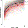
Extended Data Fig. 5 |. Variance explained by PCA and dPCA as a function of number of dimensions.

The variance explained by PCA (black) and dPCA (red) monotonically increased with the number of dimensions included. Including 10 dimensions (which the Main analyses do), PCA explained nearly all variance in neural responses (96.3%). Thin, transparent lines in the background are individual sessions. In the Main, dPCA variance explained is expressed as a fraction of PCA variance explained, as this latter one can vary considerably by brain region, and thus the variance that PCA can explain is used as a normalizing factor across brain areas.

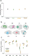
Extended Data Fig. 6 |. Stability of coupling filters across experimental blocks.

a, We compute the Pearson correlation coefficient (r) between coupling filters across a given pair of units estimated by the pGAM in leftward (80:20) and rightward-biased (20:80) experimental blocks (over 640k pairs in total). These showed a strong degree of stability (r ~0.70) and no difference across genotypes (one-way ANOVA, p = 0.79; error bars are ±1s.e.m. with the smallest n = 111,639 pairs of neurons). When separating into macro-areas (b), we observed more remapping of noise correlations in STR than the rest of areas (p < 0.05; c), but no systematic effect wherein all mouse models of ASD differed from the control. Error bars are ±1s.e.m. with the smallest n = 339 pairs of neurons.

Extended Data Fig. 7 |. Performance of the encoding model (pGAM).

We fit a coupled model (that is, with neural responses of one unit putatively impacting the firing of another) to account not solely for task-driven responses but also for internal neural dynamics. a, Comparison of $\text{pseudo-}{\mathrm{R}}^2$ for the coupled model (y axis) and an uncoupled model (x axis). Transparent dots are sessions (colored according to genotype), and opaque dots are averaged across sessions. Error bars are s.e.m. In all genotypes, the coupled model accounts better for spike trains (all p < 0.003). To assess performance of the variable selection procedure, we contrast $\text{pseudo-}{\mathrm{R}}^2$ of the models allowing for coupling, in full ($\mathrm{x}$ axis, average of 590.33 parameters) and when reduced to the variables deemed to significantly account for spiking activity ($\mathrm{y}$ axis, average of 61.25 parameters, $\alpha$ set at 0.001). b, The full and reduced models accounted for an equal portion of the variance (all p > 0.36), while the latter had a tenth of the number of parameters/retained variables.

Extended Data Fig. 8 |. Responses to contralateral and ipsilateral high contrast gratings predicted by the pGAM.

a, Evoked firing rates to high contrast gratings. As previously demonstrated (ref. 35), primary visual cortex (VISp) is particularly tuned to contralateral stimuli, while the rest of regions respond fairly equally across hemi-fields. b, Difference in the mutual information between neural responses evoked by contralateral and ipsilateral grating presentation. Error bars are ±1 s.e.m. with the smallest n = 40 neurons.

Extended Data Fig. 9 |. Peri-stimulus time histograms (PSTH) across frontal cortices as a function of sensory history.

In control animals (C57BL7, top row), neural responses were stronger to unexpected stimuli—for instance, a grating on the left hemifield (negative contrasts) under a rightward-biased block (gold color). This effect, consistent with predictive coding, was absent in Fmr1 (second row, green), Cntnap2 (third row, yellow) and Shank3 (brown) animals.

Extended Data Fig. 10 |. Sensory prediction errors as a function of cortical layer.

Sensory prediction errors are typically considered to be most common in superficial cortical layers, while silicon probes oversample deeper cortical layers. Thus, in addition to acknowledging that the method used here may not be the best suited to examine cortical sensory prediction errors, it is also possible that differences across genotypes may have arisen from a differential sampling of cortical regions. To examine this possibility, we first examined the fraction of neurons across cortical layers in each of the genotypes. a, Across the cortex as a whole, most neurons were recorded in L5 (${\chi }^2$ test, p < 0.001), followed by an approximately equal number of neurons in L2/L3 and L6 (${\chi }^2$ test contrasting L2/L3 and L6, p > 0.19). There was a nominal number of neurons in L1 and L4. This pattern was true across all genotypes (${\chi }^2$ test, p = 0.79). b, Same analysis and illustration as in a, while restricting the analysis to frontal cortical areas ACAd, ACAv and MOs. Again, there was no difference in layer sampling across genotypes (${\chi }^2$ test, p = 0.68). c, Same analyses as in b, while restricting analysis to visual cortices (VISp, VISa and VISam). There was no difference in layer sampling across genotypes (${\chi }^2$ test, p = 0.41). d, We questioned how the presence of sensory prediction errors varied across layers in FC. Unfortunately, this analysis was not possible in L1 and L4, given their very small sample sizes. Across the rest of layers (L2/L3, L5 and L6), we observe the same effect reported in the Main; presence of sensory prediction errors in C57BL7 but not mouse models of ASD (ANOVA interaction term, p < 0.001; error bars are ±1s.e.m. with the smallest n = 40 neurons). e, Prediction errors were observed in all genotypes in L2/L3 (ANOVA interaction term, p = 0.198) and not in L5 or L6 (ANOVA interaction prior block × contrast; both p > 0.71; error bars are ±1s.e.m. with the smallest n = 40 neurons).

Fig. 1 |. Reduced usage of statistical regularities in mouse models of ASD.

a, Rendering of the standardized behavioral apparatus allowing for the study of visually guided decisions in rodents. b, Schematic representation of the task. c, Performance of control (C57BL6) and mouse models of ASD (Fmr1, green; Cntnap2, yellow and Shank3, brown) on ‘easy’ trials (that is, 50% and 100% contrast) as a function of session number. Animals were considered trained when they performed at or above 80% (black dashed line) on ‘easy’ trials (moving average over three sessions). d, Psychometric functions describing the fraction of rightward choices as a function of contrast and animal genotype. Negative contrasts denote stimuli on the left. Thin and transparent lines are individual animals, while thicker and opaque lines are averages. These psychometric curves are derived by combining all sessions after animals were considered proficient (average number of trials per animal, $n=1250.9$). e, Schematic representation illustrating the ‘biased’ version of the task. The firThe verticalst 90 trials are ‘unbiased’ in that gratings appear with equal probability on the left and right (50:50). Subsequently, blocks of varying length (range = 20–100 trials, decaying exponentially such that the hazard rate was approximately constant) show gratings predominantly on the left or right (80:20 versus 20:80, respectively, in purple and gold). f, Change in the fraction of rightward responses as a function of block (rightward–leftward, fitted curves as in d), contrast and animal genotype (average number of trials per animal, $n=5645.0$). Vertical axis ($y$) in the rightmost panel is compressed to show difference between wild-type animals (black) and mouse models of ASD (colored). IR, infrared.

Fig. 2 |. Blunted accumulation of recent sensory history in mouse models of ASD.

a, Difference in cross-validated log likelihoods (that is, ‘badness’ of fit) relative to the best model (‘exp. bias’, highlighted in red). Lower is better. Description of each model in the ‘Main’. See Supplementary Fig. 2 for a different visualization of this same data, showing each individual animal. See Supplementary Fig. 3 for parameter estimates from the c.p. free run model, demonstrating that while it was a comparable fit to the exp. bias model for C57BL6 and Fmr1 animals, its resulting parameters suggest animals did not infer the presence of experimental blocks. Color scheme for genotypes follows that of Fig. 1. Error bars are ±1 s.e.m. across animals, with the smallest $n=15\text{mice}$. b, Fraction of rightward choices as a function of block (80:20 leftward in purple, 50:50 unbiased in black and 20:80 rightward in gold) for four example animals; one per genotype. Circles are data, and lines are fits from the exp. bias model. c, Example fits of the exp. bias model (lines) when plotting data as a function of trials to and since block change (in this case, from 80:20 to 20:80). As expected, behavior change is most notable for 0 contrast trials (colored). The rest of contrasts are grouped, with the color gradient (from dark to light blue) following the spectrum from strong evidence for left targets to right targets. d, Visualization of the average exponential decay (top) and $\beta$ hyper-priors (bottom) dictating the exp. bias model for wild-type (black) and mouse models of ASD (colored). The hyper-priors being taller and narrower in ASD result in a diminished change in the subjective prior with changing environmental statistics. PDF, probability density function. e, Illustration of an experimental sequence of trials; the experimentally imposed probability that the stimuli will be on the left (black step functions), what an optimal observer would be able to infer (gray) and the best estimates of subjective priors for the average control animal (top; black jagged line), as well as the average Fmr1 (top; green), Cntnap2 (middle; yellow) and Shank3 (bottom; brown) animal. f, Subjective prior before and after block changes in the wild-type (black) and mouse models of ASD (colored). Estimates are baseline-corrected averages across animals and all transitions. Error bars represent ±1 s.e.m. C.p., change point.

Fig. 3 |. A large-scale neurophysiological survey across mouse models of ASD.

a, Reconstruction of probe locations for the different genotypes (C57BL6, black; Fmr1, green; Cntnap2, yellow and Shank3, brown). b, Number of units recorded per area ($y$ axis; subset shown) and genotype. Bars are filled and opaque if all genotypes had at least 40 units in that area, filled and transparent if the given genotype had 40+ units but others did not and empty if less than 40. c, Raster plot (top) and PSTH (bottom) to stimulus onset for example units in VISp. Raster is sorted by contrast (positive values indicating gratings presented on the right; recordings on the left hemisphere; a). d, Similar to c but showing responses in anterior cingulate area, dorsal part (ACAd). e, Raster and PSTH to stimulus onset, but sorted as a function of choice. Areas are marked on the top left of raster plots. f, Similar to c–e, but sorted by alignment to feedback onset and sorted as a function of correct and incorrect responses. g, Example spike counts (normalized; colored by genotype) before stimulus onset (−300 to −50 ms) as a function of trial number (x axis). Also plotted are the experimentally imposed prior and the subjective estimate of the prior for the given animal per session. Right, we highlight example periods where the firing rate changes during changes in the subjective prior and stable experimental prior in gray color.

Fig. 4 |. Population encoding of subjective prior shifts from visual to FC in mouse models of ASD.

a, Four example dPCA sessions, one per genotype. Analysis was conducted to separate quintiles of the subjective prior and left versus right decision. Top row shows a ‘condition-independent’ subspace capturing the stimulus-evoked response (only left decision—solid lines—shown for clarity). Middle row shows the decision subspace appropriately separating left (solid line) and right (dashed line) choices. Bottom row shows the subjective prior subspace. Of note, the quintiles of the subjective prior are differentiated before the stimulus is presented (x axis = 0). b, Categorization of brain regions into ‘macro-areas’ for statistical power and coarse summary (see Supplementary Table 1 for further detail on the categorization). c, Variance explained by the subjective prior subspace as a function of ‘macro-area’ and mouse genotype (C57BL6, black; Fmr1, green; Cntnap2, yellow and Shank3, brown). Error bars represent ±1 s.e.m. with the smallest $n=13$ (macro-area–genotype pair). See Supplementary Fig. 5 for an alternative illustration showing all sessions. STR, striatum.

Fig. 5 |. Unit encoding of subjective prior shifts from visual and frontal cortices in mouse models of ASD.

a, Schematic representation of the pGAM encoding model. b, Example units showing the empirical PSTH (black, $x$ axis is time), the reconstructed average from the pGAM (red) and the (exponentiated) visual stimulus kernel (blue). The latter is the contribution to the observed response that the encoding model ascribes (factorized) to visual stimulus presentation. c, Example tuning function to the subjective prior. Follows the format from b, with the difference that the $x$ axis is not time anymore, but the value taken by the subjective prior. The $x$ axis is normalized such that the lowest value taken during a recording (y axis in Fig. 2b) takes a value of 0 and the maximum takes a value of 1. By definition, therefore, 0.5 corresponds to the average subjective prior of the animal. d, Fraction of units significantly tuned ( $P<0.001$) to the subjective prior as a function of brain region (vertical; see Allen CCF for acronyms) and genotype (C57BL6, black; Fmr1, green; Cntnap2, yellow and Shank3, brown). e, Follows the convention from d, showing the informativeness of tuning functions (measured in MI). Error bars are ±1 s.e.m, with the smallest $n=40$ neurons. ProS, prosubiculum; SUB, subiculum; LD, lateral dorsal nucleus; LGd, lateral geniculate nucleus, dorsal part; PO, posterior thalamic nuclear group; CP, caudoputamen; LS, lateral septal nucleus; MRN, median raphe nucleus; PRT, pretectal region; SF, subfornical organ.

Fig. 6 |. Outsized coding of deviations from long-run prior across mouse models of ASD.

a, Two-dimensional t-SNE of tuning functions to the subjective prior as a function of brain area (colors). Inset shows the average and s.e.m. silhouette values (that is, relative distance of points to others within and across clusters) as a function of a number of clusters. A high silhouette value indicates that points within a cluster are well matched to their own cluster and poorly matched to other clusters. b, Examples (thin and transparent) and average (dark and opaque) tuning functions to the subjective prior as a function of cluster (one through four). c, Left, fraction of the units tuned to the subjective prior that belong to each of the four clusters (shown in b) as a function of genotype (rows; C57BL6, Fmr1, Cntnap2 and Shank3, respectively). Right, fraction of units increasing their firing rate with decreasing (left—red) versus increasing (left—blue) value of the subjective prior (gray), and fraction of units increasing their firing rate with increasing (left—green) versus decreasing (left—purple) distance from the long-run prior (that is, normalized subjective prior = 0.5). d, Fraction of cluster 1/cluster 2 (gray in c) as a function of genotype (colors) and macro-brain area. Acronyms follow the convention from Fig. 4. e, As d, showing the fraction of cluster 3/cluster 4. The dashed line shows a fraction = 1.

Fig. 7 |

Lack of sensory-driven prediction errors in FC of mouse models of ASD. MI ($y$ axis) as a function of grating contrast (y axis; negative contrasts are gratings presented on the left hemifield), experimental block (leftward bias block in purple, 80:20), macro-area (columns) and genotype (rows). Error bars are ±1 s.e.m, with the smallest $n=40\text{neurons}$.

Fig. 8 |. FC surprise responses reflect the computational anomaly and reduced prior encoding.

a, Regression coefficients (left) and P values (right) associated with coefficients from a multiple regression of the form $y~\mathrm{i}\mathrm{n}\mathrm{t}\mathrm{e}\mathrm{r}\mathrm{c}\mathrm{e}\mathrm{p}\mathrm{t}+{\beta }_1{x}_1+{\beta }_2{x}_2\dots {\beta }_n{x}_n$, where $y$ is the sum of the parameters dictating the shape of the hyperprior $\beta$ distribution (that is, sum of $\alpha +\beta$), which leads mouse models of ASD toward ‘conservatism’, and the $x$’s are shown along the rows and columns of b. The only significant coefficient ( $P<0.05$) was the degree of surprise responses (that is, sensory prediction error) in FC. This coefficient was negative (that is, less FC surprise correlates with more conservatism), while the rest of the coefficients in FC were positive. b, Correlation matrix between the coefficient inputs in a. $R$ values are plotted color coded as a function of whether correlations were positive (red) or negative (blue). Asterisks indicate $P$ values < 0.05 with Bonferroni correction. The matrix is symmetrical vis-à-vis the diagonal, and thus asterisks are only marked on the lower half. For visualization, each area (CA, MOp, FC and VIS) is highlighted in a black box, and correlations within area with the magnitude of surprise responses are highlighted in green.

References

1. Gaugler T et al. Most genetic risk for autism resides with common variation. Nat. Genet. 46, 881–885 (2014). - PMC - PubMed
1. Krumm N et al. Excess of rare, inherited truncating mutations in autism. Nat. Genet. 47, 582–588 (2015). - PMC - PubMed
1. Iakoucheva LM, Muotri AR & Sebat J Getting to the cores of autism. Cell 178, 1287–1298 (2019). - PMC - PubMed
1. Satterstrom FK et al. Large-scale exome sequencing study implicates both developmental and functional changes in the neurobiology of autism. Cell 180, 568–584 (2020). - PMC - PubMed
1. American Psychiatric Association. Diagnostic and Statistical Manual of Mental Disorders. Fifth Edition (American Psychiatric Association, 2022).