Visualizing dynamics of charges and strings in (2 + 1)D lattice gauge theories

Abstract

Lattice gauge theories (LGTs)^1-4 can be used to understand a wide range of phenomena, from elementary particle scattering in high-energy physics to effective descriptions of many-body interactions in materials^5-7. Studying dynamical properties of emergent phases can be challenging, as it requires solving many-body problems that are generally beyond perturbative limits^8-10. Here we investigate the dynamics of local excitations in a $Z_2$ LGT using a two-dimensional lattice of superconducting qubits. We first construct a simple variational circuit that prepares low-energy states that have a large overlap with the ground state; then we create charge excitations with local gates and simulate their quantum dynamics by means of a discretized time evolution. As the electric field coupling constant is increased, our measurements show signatures of transitioning from deconfined to confined dynamics. For confined excitations, the electric field induces a tension in the string connecting them. Our method allows us to experimentally image string dynamics in a (2+1)D LGT, from which we uncover two distinct regimes inside the confining phase: for weak confinement, the string fluctuates strongly in the transverse direction, whereas for strong confinement, transverse fluctuations are effectively frozen^11,12. We also demonstrate a resonance condition at which dynamical string breaking is facilitated. Our LGT implementation on a quantum processor presents a new set of techniques for investigating emergent excitations and string dynamics.

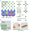
Fig. 1. An LGT and its phase diagram.

a, A full two-dimensional LGT (top left) can be realized by placing charged matter (grey circles) on vertices of a square lattice and gauge fields on the links between them (green diamonds). The local gauge structure can be used to eliminate the matter field and arrive at an effective theory involving gauge fields only (right). The presence/absence of charge excitations (red/blue) or magnetic fluxes (yellow/purple) is then sensed through the links. b, Zero-temperature phase diagram of the LGT in equation (1). c, In the deconfined phase, charges move freely. In the confined phase, charges oscillate around an equilibrium configuration. We can picture an elastic string connecting them that fluctuates in both longitudinal and transverse directions, limiting their motion.

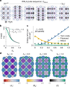
Fig. 2. WALA.

a, WALA gate sequence used for a two-dimensional grid of 35 qubits, consisting of 17 link qubits (diamonds) and 18 ancilla qubits (circles). The sequence begins with applying R_y(θ) to ancilla qubits of each plaquette, followed by applying C-NOT gates to qubit pairs, starting at the centre columns and moving outwards. b, Optimized θ angle used in WALA. The green curve is based on numerical calculations for a 35-qubit grid and the grey curve shows the thermodynamic limit. c, Energy error, compared with the exact ground state, of three ansatzes: (1) WALA (green); (2) toric code, θ = π/2 (blue); and (3) product state, |0⟩^⊗N (yellow), for λ = 0.25. Solid lines correspond to circuit simulations and filled circles are extracted from our experiment after readout error mitigation (Supplementary Information Section III.A). d, Experimentally measured expectation values of plaquette, vertex and Pauli-Z operators, for λ = 0.25 and h_E ∈ {0, 0.3, 0.6, 1.0}, from WALA. We post-select the measured data on the ancilla being in the expected |0⟩ state to mitigate decoherence of the device for this and all other figures of the main text (Methods).

Fig. 3. Confinement of electric excitations.

a, A Pauli-X gate applied to the WALA initial state creates two electric excitations on adjacent vertices (red tiles). The coupling induces dynamics to the excitations and is set to λ = 0.25 for all data in this figure. After post-selecting bitstrings that correspond to two electric excitations, the separation of the excitations is monitored as a function of time for different electric fields h_E. The grey area is bounded by the separation measured when evolving under the pure toric code Hamiltonian (λ = h_E = 0). The lower panel shows the rescaled data, assuming a global depolarizing noise channel, and compares it with exact circuit simulation. b, Average density of electric excitations as measured by ⟨A_v⟩ for h_E = 0 (left) and h_E = 2.0 (right). c, Two superposition states in which the excitations interfere constructively (|ψ₊⟩) and destructively (|ψ₋⟩) at short distances, respectively. d, The separation of the excitations as a function of time for different electric fields h_E. Lines represent guides for the eye. All error bars in this work show standard deviation of the mean and are smaller than the markers when not visible. e, Spatial maps of the probability that an electric vertex A_i,j is excited, conditioned on the electric vertex being excited at time t = 3.5: P(i, j|). The different columns correspond to different , indicated by the boxed symbols. The unconditioned probability that is excited is written below the symbol. The colour scale represents P(i, j|) for all i and j. The top and bottom rows show results for h_E = 0 and 2.0, respectively. We implement dynamical decoupling and randomized compiling to mitigate control errors, as well as idle dephasing (Methods).

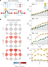
Fig. 4. Dynamics of the string connecting two spatially localized electric charges.

a, Schematic of the initial state preparation. Starting from the WALA initial state as vacuum, we create a pair of separated electric excitations by applying a string of X gates spanning from an extra qubit on the left (leftmost diamond) to one on the right (rightmost diamond). By not applying the local field terms of the time evolution on those two extra qubits, the excitations remain pinned, whereas the string itself can evolve dynamically. b, Circuit for measuring the unequal-time correlation function Re[⟨Z(t)Z(0)⟩]. The P gate is H(S^†)^b, in which b = 0/1 corresponds to measuring the real/imaginary part of ⟨Z(t)Z(0)⟩. The CZ gate entangling the auxiliary qubit (Q_b) to the gauge qubit of interest (Q_l) may need to be mediated by means of swaps through an ancillary qubit (Q_a) and another gauge qubit (Q_g). c, Spatial maps of ${\mathcal{S}}_{ZZ}\left(t\right)=\mathrm{Re}\left[⟨Z\left(t\right)Z\left(0\right)⟩\right]\times ⟨Z\left(0\right)⟩$ for varying times and confining field h_E, at λ = 0.25 and dt = 0.3 (the same for all data in the figure). The extra qubits on either side used for state preparation are not shown. d, Re[⟨Z(t)Z(0)⟩] and ${\mathcal{S}}_{ZZ}\left(t\right)$ for qubits Q₁ and Q₂ in the centre-top and centre-bottom respectively, as labelled in panel c. Lines are guides for the eye. The grey regions in these plots correspond to the region limited by decoherence and is bounded by $\mid ⟨Z\left(t\right)Z\left(0\right)⟩{\mid }_{\lambda =h_{\mathrm{E}}=0}$.

Fig. 5. String breaking.

a, Schematics for pair creation from vacuum fluctuation and string breaking. b, Difference in the charge excitation values in the presence and absence of the string ⟨A_v⟩_string − ⟨A_v⟩_vacuum, for λ ∈ {0, 0.25, 0.50} at h_E = 1.4 and t = 2.7, with dt = 0.3. c, Probability of a vertex excitation P(A_v) on three distinct vertices A₁ (gold), A₂ (green) and A_vac (black) for λ ∈ {0, 0.25, 0.50} and h_E = 1.4. The grey ‘decoherence-limited’ region is defined by the average of P(A_v) over all vertices having evolved the initial state with the X string for λ = 0, h_E = 1.4. d, Dependence of P(A_v) on h_E, acquired at t = 2 (dt = 0.2), for λ = 0 (pluses), λ = 0.25 (crosses) and λ = 0.50 (pentagons).

Extended Data Fig. 1. Qubit grid and experimental fidelities.

a, Grid of 45 qubits used in this work. Green diamonds represent physical gauge qubits, grey circles are the ancilla qubits used in Trotterized time evolution and blue circles are the ancilla qubits used in projective state preparation and Hadamard test experiments. b, Representative cumulative distribution functions of relevant gate and measurement errors. Single-qubit Clifford and non-Clifford Pauli errors, determined from randomized benchmarking, are shown in red and orange with median errors of 0.100% and 0.095%, respectively. To implement non-Clifford randomized benchmarking, we replace the standard depth-n randomized benchmarking sequence, which consists of n − 1 random Clifford gates and a final Clifford gate that inverts the sequence, with $U_f{\mathrm{XU}}_{\frac{n-1}{2}}\dots X{U}_0$, in which each U_i is a Haar random single-qubit unitary and U_f is computed to invert the whole sequence. The error rate thus obtained, which includes approximately equal contributions from the Clifford X gates and the non-Clifford U_i gates, is what is plotted in panel b as ‘1Q non-Clifford’. Inferred CZ Pauli errors, determined from cross-entropy benchmarking, for all pairs are shown in blue with a median error of 0.52%. |0⟩ state and |1⟩ state readout errors, determined from sampling random bitstrings, are shown in green and olive with median errors of 0.60% and 2.00%, respectively.

Extended Data Fig. 2. Suzuki–Trotter evolution circuit.

Trotterized time evolution follows initial state preparation (Fig. 2). The Trotter cycle is broken into single-qubit field terms, which act on the individual physical qubits, and plaquette terms, which involve four layers of C-NOT gates on each vertex and plaquette, single-qubit rotations on all ancilla qubits and a subsequent four layers of C-NOT gates to disentangle the ancilla qubits from the physical ones.

Extended Data Fig. 3. Post-selecting on measured ancilla state.

a, Heatmaps showing the probability of measuring the ancillas in the |1⟩ state, $⟨P_{Z_l}⟩$, at times t ∈ {0.5, 2.5, 4.5} (dt = 0.5). A representative value of h_E = 0.6, λ = 0.25 was chosen. b, $⟨P_{Z_l}⟩$ traces for all qubits (transparent traces) and their average (dark-green line). c, Number of total shots collected and post-selected shots as a function of evolved time. Grey points show the number of post-selected shots based on all ancillas being measured in the |0⟩ state. The red points indicate the number of shots after also post-selecting on the two-excitation sector. The black points show the prediction of post-selected shots assuming that the system was in the maximally mixed state (negligible). The green dotted line (right axis) shows the total number of shots collected for each time step. d, Separation between two excitations, starting from the initial state shown in Fig. 3a, following evolution under the pure toric code Hamiltonian. Green markers show the separations when averaging over all bitstrings, regardless of the final state of the ancilla qubits. The red markers only average over instances when all ancilla qubits were measured in the |0⟩ state. The theoretical expectation for the distance is constant at 1 (solid black line), whereas the expectation value for the maximally mixed state is 7/3 (dotted line).

Extended Data Fig. 4. Local and global depolarization comparison with quantum processor data.

a, Separation between excitations, after starting with excitations a distance 1 apart on a 2 × 3 vertex lattice. Trotter evolution with λ = 0.25 and h_E ∈ {0, 0.25, 2.25} are shown for device data (markers), simulations with local depolarizing noise (dashed lines) and with global depolarizing noise (solid lines). b, Data for evolution of the same initial state but with Trotter evolution with λ = 0, at which the vertex excitations should be stationary. The distance in the noiseless case should be 1 (solid line), whereas the expectation of distance for the maximally mixed state is 5/3 (dashed line). c, The extracted global depolarizing probability for the data in panel b.

Extended Data Fig. 5. The variational circuit ansatz and transforming the original Hamiltonian with the C-NOT gates of the variational circuit.

This circuit is equivalent to the one in the main text but does not use ancilla qubits. a, The unitary applied on each plaquette consists of two parts: First, a single-qubit y-rotation gate R_y(θ) = exp(−iθY/2) with variational parameter θ is applied to the top qubit of the plaquette. Then, three C-NOT gates are applied, with the top qubit being the control qubit and the other qubits being the targets. b, The order of the plaquette unitaries is chosen such that the y-rotation gate always acts on a |0⟩ state. Here the blue diamonds denote the gate in a; lighter coloured gates are applied first and darker coloured gates last. The order of plaquettes is also indicated by the grey arrow. c, The original Hamiltonian is drawn schematically on a lattice of 4 × 4 vertex operators. The orange terms connecting Pauli-Zs denote the different vertex operators of the Hamiltonian, the blue terms connecting Pauli-Xs denote the plaquette operators and the green Pauli-Zs denote the onsite Z-field. d, After conjugating each term in the Hamiltonian by the C-NOT layer of the circuit, we arrive at a new Hamiltonian. The orange vertex operators have been transformed to Ising terms, the blue plaquette operators have been transformed to single-site Pauli-X terms and the green Pauli-Z terms have been transformed to two-site or three-site Pauli-Z operators. On all sites at which no Pauli-X operator acts, the Hamiltonian commutes with single-site Pauli-Z operators, so on those sites, the eigenstates of the Hamiltonian are either in the |0⟩ or the |1⟩ state. e, In the subspace in which all qubits except the top qubit on each plaquette are in the |0⟩ state, the transformed Hamiltonian turns into a two-dimensional transverse-field Ising model.

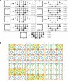
Extended Data Fig. 6. Operator transformations on a single plaquette and plaquette-by-plaquette transformation of the Hamiltonian.

a, The table shows the different transformations of the operators on a plaquette when transforming them with the C-NOT gates of the variational circuit acting on that plaquette. The left side shows the transformations of the different vertex operators. Note that, when a vertex operator has some remaining Z gates not supported on this specific plaquette, they are left unchanged by the C-NOT gates. The right side shows the transformations of the different onsite Pauli-Z operators. The last diagram at the bottom shows the transformation of the plaquette operators. b, We can use the results of the table in a to transform the original Hamiltonian plaquette by plaquette. At each step, the plaquette transformed next by the C-NOT gates in the variational circuit is highlighted in yellow. Note that the plaquettes of the Hamiltonian are transformed in the opposite order of how they are applied in the quantum circuit in Extended Data Fig. 5b. Because the C-NOT gates in the circuit applied to plaquettes in the same row commute, we can transform a whole row of the Hamiltonian at the same time.

Extended Data Fig. 7. Average expectation values of terms in H for the WALA.

Expectation values of each term in the Hamiltonian, averaged over all equivalent vertices/plaquettes/links. For the expectation values of links, ⟨Z_l⟩ is expected to behave differently for qubits on the edge and those in the bulk (Methods). Therefore, we plot the average expectation values for these two sets of qubits separately. The expectation values are plotted for electric vertices ⟨A_v⟩ (blue markers), magnetic plaquettes ⟨B_p⟩ (purple markers), external edge links ⟨X_l⟩_ext and ⟨Z_l⟩_ext (dark green and black markers, respectively) and internal bulk links ⟨X_l⟩_int and ⟨Z_l⟩_int (light green and grey markers, respectively). Error bars correspond to the standard deviation over all vertices, plaquettes or links.

Extended Data Fig. 8. Average heatmaps and conditional probabilities for the superposition initial states.

a, Schematic showing the preparation of the superposition initial states. Such a circuit produces a mixed state, which can be projected on |ψ₊⟩ or |ψ₋⟩ depending on the measurement of the ancilla qubit Q_b. Qubits defined in b. b, Temporal evolution of average heatmaps of ⟨A_v⟩ for the |ψ₋⟩ state, with h_E ∈ {0, 2.0}. The grey value of  +2/3 on the colour bar corresponds to the average value when two electric excitations are equally distributed across the entire grid. For this figure, λ = 0.25. c, Temporal evolution of average heatmaps of ⟨A_v⟩ for the |ψ₊⟩ state, with h_E ∈ {0, 2.0}. d, Conditional excitation location probabilities for the |ψ₊⟩ state, after post-selecting on the two-excitation sector, at time t = 3.5. The grey region of the colour bar corresponds to the average value when the excitation not conditioned on is equally distributed across the entire grid. The numbers inside the measurement boxes show the unconditioned probability of measuring an electric excitation on that site. e, Excitation separation for both |ψ_±⟩ initial states and h_E ∈ {0, 2.0}. The markers show measured data (reproduced from Fig. 3). The lines show noiseless numerical circuit simulations.

Extended Data Fig. 9. Measurements of ⟨Z(0)⟩, Im[⟨Z(t)Z(0)⟩] and ⟨Z(t)⟩.

a, Measured expectation values of ⟨Z(0)⟩ after preparing the WALA ground state with a string excitation as in Fig. 4a (top panel). The short-circuit depth for state preparation leads to excellent agreement with numerical simulations without any error mitigation (bottom panel). b, Measured expectation values of Im[⟨Z(t)Z(0)⟩] for Q₁ and Q₂, defined in Fig. 4 (top panels). Data points were acquired using dt = 0.3 and λ = 0.25. The grey areas on these plots correspond to the region limited by decoherence and is bounded by $\mid ⟨Z\left(t\right)Z\left(0\right)⟩{\mid }_{\lambda =h_{\mathrm{E}}=0}$. This is then used to rescale the data to compare with noiseless numerical simulations using a global depolarizing model as described in Methods (bottom panels). c, Measured expectation values of ⟨Z(t)⟩ for Q₁ and Q₂ (top panels). The grey areas on these plots correspond to the region limited by decoherence and is bounded by ⟨Z(t)⟩ of the WALA initial state under evolution of the pure toric code Hamiltonian. This is then used to rescale the data to compare with noiseless numerical simulations using a global depolarizing model (bottom panels).

Extended Data Fig. 10. Build-up of vertex excitations with and without an initial string.

a, Spatiotemporal map of ⟨A_v⟩ for three different λ ∈ {0, 0.25, 0.50} and constant h_E = 1.4, starting from the WALA initial state and time evolving. b, Same as panel a but starting with an excited initial state with a string stretched across the grid, whose initial trajectory is indicated by the black qubits. c, The average probability of finding a vertex excitation on any site, for each of the columns in panels a and b (both initial states). Results from evolving the WALA initial state are shown in beige and those from evolving the string initial state are shown in dark green. Markers represent experiments with λ = 0 (pluses), λ = 0.25 (crosses) and λ = 0.50 (stars). The grey region is bounded by the average of all vertices when λ = 0 having started in the initial state (same as green pluses). The bottom panel shows the global depolarization rescaled values (markers) and the numerical noiseless circuit simulations (lines).

References

1. Wegner, F. J. Duality in generalized Ising models and phase transitions without local order parameters. J. Math. Phys.12, 2259–2272 (1971).
1. Wilson, K. G. Confinement of quarks. Phys. Rev. D10, 2445 (1974).
1. Kogut, J. & Susskind, L. Hamiltonian formulation of Wilson’s lattice gauge theories. Phys. Rev. D11, 395 (1975).
1. Kogut, J. B. An introduction to lattice gauge theory and spin systems. Rev. Mod. Phys.51, 659 (1979).
1. Weinberg, S. The Quantum Theory of Fields (Cambridge Univ. Press, 1995).
LinkOut - more resources