Geospatial analysis of toponyms in geotagged social media posts

Abstract

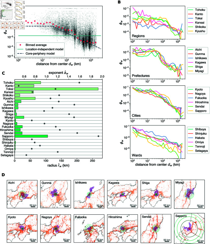
Place names, or toponyms, play an integral role in human representation and communication of geographic space. In particular, how people relate each toponym with particular locations in geographic space should be indicative of their spatial perception. Here, we make use of an extensive dataset of georeferenced social media posts, retrieved from Twitter, to perform a statistical analysis of the geographic distribution of toponyms and uncover the relationship between toponyms and geographic space. We show that the occurrence of toponyms is characterized by spatial inhomogeneity, giving rise to patterns that are distinct from the distribution of common nouns. Using simple models, we quantify the spatial specificity of toponym distributions and identify their core-periphery structures. In particular, we find that toponyms are used with a probability that decays as a power law with distance from the geographic center of their occurrence. Our findings highlight the potential of social media data to explore linguistic patterns in geographic space, paving the way for comprehensive analyses of human spatial representations.

Fig 1. Places in Japan denoted by the toponyms studied in this paper.

In this study, we sample 24 toponyms: the names of (A) six regions, (B) six prefectures, (C) six major cities, and (D) six wards (submetropolitan/submunicipal districts). The colored areas in each panel show the administratively defined geographic area (except for cities) denoted by each toponym. (A) The extent of each region is not uniquely defined. Here we show one of the commonly used classifications of regions. (C) The colored area shows the metropolitan employment area [23, 24], which is considered to be more representative of urban activity than administratively defined city areas. Note that Kyoto, Hiroshima, and Fukuoka are used both as the names of the cities and as the names of the prefectures of which the cities are the capitals. (D) Prefectural boundaries are shown for visual guidance. Maps made with Natural Earth (https://www.naturalearthdata.com/).

Fig 2. The spatial densities of geotagged posts, resident population, and employed population.

(A–C) Geographic distribution of the three densities. Note that the population data are geographically limited inside Japan, while the geotagged posts are sampled in the bounding box of Japan, which also includes neighboring countries. Maps made with Natural Earth (https://www.naturalearthdata.com/). (D) Probability distribution of density (the number of geotagged posts per unit area). (E, F) Scatter plots showing the correlation between each of the population densities and the geotagged post density. Pearson and the Spearman correlation coefficients are shown below the plot. (G) Probability distributions of the three densities, each rescaled by its mean.

Fig 3. Occurrence pattern of Fukuoka.

(A) Geographic distribution of density ${\sigma }_w$. (B) Geographic distribution of occurrence ratio ${\varphi }_w$. (C) Probability distributions of spatial density for all geotagged posts (in gray) and for Fukuoka (in blue). (D) Scatter plot showing the relationship between the total number of geotagged posts $n_{\mathrm{a}\mathrm{l}\mathrm{l}}$ and the number of posts containing Fukuoka n_w in each grid cell. The lines represent contours along which the density of points (kernel density estimate) on the double logarithmic scale is constant. The region inside each contour, from dark to light colors, contains 90.0%, 99.0%, and 99.9% of the data points, respectively. (E) The same scatter plot as panel D, but with points colored by the distance between the grid cell and the center O_w. Maps made with Natural Earth (https://www.naturalearthdata.com/).

Fig 4. Relationship between n_w and nall in empirical and model distributions.

(A) Scatter plots for different keywords. (B, C) Kernel density profiles of empirical and model distributions. In each panel, the red contours show the density profile obtained from the location-independent model (B) or the core-periphery model (C), fitted to the empirical occurrence pattern of each word, represented by the blue contours. As in Fig 3D, the region inside each contour, from dark to light colors, contains 90.0%, 99.0%, and 99.9% of the data points, respectively. Note that the scatter plot of empirical data and its density profile for Fukuoka are identical to those in Fig 3D.

Fig 5. Dissimilarity of empirical data from the location-independent model.

The dissimilarity is evaluated by relative entropy $D_{\mathrm{K}\mathrm{L}}({\tilde{Q}}_w\parallel P_w)$. For each word, 3000 grid cells are randomly sampled 50 times. The error bar shows the 95% confidence interval.

Fig 6. Core-periphery patterns of toponym occurrence.

(A) Occurrence ratio ${\varphi }_w$ of Fukuoka against distance d_w from center O_w (small black dots), overlaid with the average for each logarithmic bin (red circles). The solid and dashed lines represent the maximum likelihood fits of the location-independent and core-periphery binomial models. (B) Average occurrence ratio as a function of d_w for all the domestic toponyms studied in this work. (C) Maximum likelihood estimator of the core-periphery model parameters for each toponym. We represent estimated radius ${\hat{r}}_w$ by bars colored according to the category of the toponym (lower axis) and estimated exponent ${\hat{a}}_w$ by gray circles (upper axis). The standard errors are omitted as they are too small to be meaningfully visualized. (D) The fitted core-periphery model compared to the administrative/metropolitan area. The innermost circles in dark green represent the core boundary (distance r_w from the center O_w) and the two outer circles in lighter green denote the distance at which the occurrence probability p_w,c is equal to one half and one third of the probability in the core q_w, respectively. The areas shaded in purple indicate the administrative area of each prefecture (top row) and the metropolitan employment area of each city (bottom row). Maps made with Natural Earth (https://www.naturalearthdata.com/).

Fig 7. A schematic diagram of the core-periphery model.

Top: The occurrence probability p_w,c of toponym w at grid cell c is equal along each contour line. The model is isotropic in geographical space, meaning the equiprobability lines form concentric circles centered at O_w. The inside of inner most circle of radius r_w is the core. Bottom: The occurrence probability profile. Inside the core, p_w,c is constant at q_w, while it decays outside the core as a power law with exponent a_w as a function of distance d_w,c from O_w.

Fig 8. Goodness of fit evaluated by Akaike information criterion (AIC).

References

-
- Montello DR, Goodchild MF, Gottsegen J, Fohl P. Where’s downtown?: Behavioral methods for determining referents of vague spatial queries. Spatial Cognit Comput. 2003;3(2–3):185–204. doi: 10.1080/13875868.2003.9683761 - DOI
- Jones CB, Purves RS, Clough PD, Joho H. Modelling vague places with knowledge from the Web. Int J Geograph Inf Sci. 2008;22(10):1045–65. doi: 10.1080/13658810701850547 - DOI
- DeLozier G, Baldridge J, London L. Gazetteer-independent toponym resolution using geographic word profiles. AAAI. 2015;29(1):2382–8. doi: 10.1609/aaai.v29i1.9531 - DOI
- Cheng Z, Caverlee J, Lee K. You are where you tweet. In: Proceedings of the 19th ACM International Conference on Information and Knowledge Management. ACM. 2010. doi: 10.1145/1871437.1871535 - DOI
- Li W, Serdyukov P, de Vries AP, Eickhoff C, Larson M. The where in the tweet. In: Proceedings of the 20th ACM International Conference on Information and Knowledge Management. ACM. 2011. doi: 10.1145/2063576.2063995 - DOI
MeSH terms
LinkOut - more resources
Full Text Sources