Intercellular communication in the brain via dendritic nanotubular network

Abstract

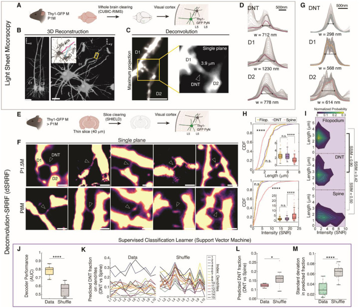
Recent studies have identified intercellular networks for material exchange by bridge-like nanotubular structures, yet their existence in neurons remains unexplored within the brain. Here, we identified long, thin dendritic filopodia that establish direct dendrite-to-dendrite contacts, forming dendritic nanotubes (DNTs) in mammalian brains. Using super-resolution microscopy, we characterized their unique molecular composition and dynamics in dissociated neurons, enabling Ca²⁺ propagation over distances. Utilizing imaging and machine-learning-based analysis, we confirmed the in situ presence of DNTs connecting dendrites to other dendrites whose anatomical features are distinguished from synaptic dendritic spines. DNTs mediate the active transport of small molecules or human amyloid-beta (Aβ), implicating the role of DNT network in AD pathology. Notably, DNT levels increased prior to the onset of amyloid plaque deposits in the mPFC of APP/PS1 mice. Computational simulations predicted the progression of amyloidosis, providing insight into the mechanisms underlying neurodegeneration through these DNTs. This study unveils a previously unrecognized nanotubular network, highlighting another dimension of neuronal connectivity beyond synapses.

Figure 1.. Dendritic nanotubes (DNTs) in dissociated cortical neurons

(A) Representative image of live cortical neurons in dissociated culture (DIV9) by dSRRF microscopy which visualizes neuronal membrane (NeuO, green) and microtubule (SiR-tubulin, magenta). n_volume = 100 for dSRRF reconstruction. (B) Interextensions between two neurites (branched directly from somas or other neurites) shown in conventional (top) and dSRRF (bottom) microscopies, magnified from the boxed region (yellow) in (A). Cross-sectional intensity profiles averaged from colored boxes (left) show distinct cytoskeletal composition between interextensions. (C) Signal-to-noise ratio (SNR) of averaged intensity profile along structures, which normalized by width (FWHM; Full Width at Half Maximum) for each cytoskeletal component from tubulin-negative (left, n = 230; SNR_tubulin < 1.2) and tubulin-positive (right, n = 995; SNR_tubulin ≥ 1.2) interextensions. P = 2.9 × 10⁻²⁶ between groups by unbalanced two-way ANOVA. The fraction of each group was represented (top, mean ± s.d.; n_FOV = 59). (D) Width of structures (n = 230 and 995 for (−) and (+) tubulin; P = 1.6 × 10⁻¹³ by two-tailed unequal variances t-test). (E) Representative multicolor dSRRF image of fixed cortical neurons in dissociated culture (DIV14) with staining of three cytoskeletal proteins of F-actin (green), neurofilament (pNF-H, blue), and tau (red). n_volume = 1,000 for dSRRF reconstruction. (F) Interextensions between two neurites in dSRRF microscopies, magnified from the boxed region (yellow) in (E), and their cross-sectional intensity profiles. (G) Another example of an interextension linking a soma and a neurite (left), its axial montage (right, top), and cross-sectional intensity profile (right, bottom). (H) Percentage of F-actin-only structures in interextensions and neurites (n_FOV = 11) whose SNR for pNF-H and tau < 1.2 (two-tailed unequal variances t-test, P = 1.2 × 10⁻¹⁰). (I) SNR of averaged intensity profile along structures, normalized by width for each cytoskeletal component from F-actin-only intermextensions (left, n = 302), composite interextensions (middle, n = 452), and neurites (right, n = 191). P = 8.9 × 10⁻¹² for Actin-IB vs. Comp-IB, P = 1.7 × 10⁻⁹ for Actin-IB vs. Primary, and P = 0.80 for Comp-IB vs. Primary by unbalanced two-way ANOVA, P = 2.0 × 10⁻¹³ among groups. (J-K) Width and length of structures (P = 0.0036 for Actin-IB vs. Comp-IB, P = 0 for Actin-IB vs. Primary, and P = 0 for Comp-IB vs. Primary by one-way ANOVA; P = 1.9 × 10⁻⁹⁸ for (J), P = 0.95 for Actin-IB vs. Comp-IB by two-tailed unequal variances t-test for (K)). (L) Representative images displaying formation (top) and extinction (bottom) of interextensions from and to filopodia observed in time-lapse imaging of NeuO-stained neurons for 2 hours (video rate = 1 min). (M) Percentages of interextension formation connecting neurites (N-N) or a neurite and a soma (N-S) by filopodial contact or another mechanism (i.e. shaft contact) on DIV3.5 and DIV7 (n_exp = 37 and 35; n_event = 46 and 18; Filopodial formation = 93 % and 83 % for DIV3.5 and DIV7 respectively). (N) Temporal stability of interextensions (top; n = 59) and primary neurites (bottom; n = 73) is shown by percentages of structures presented longer or shorter than 4 hours in time-lapse imaging (66 hours, video rate = 15 min) of cortical neurons stained by 100 nM SiR-actin. (O-Q) The pharmacological effects of interextension formation from filopodia in time lapse imaging (1-hour-long, video rate = 1 min). The numbers of active filopodia (O), formation events (P), and extinction events (Q) were counted in the FOV (87 × 87 μm²) after 60-min-long incubation with 0.1% DMSO (n_FOV = 23), 2 μM Rotenone (n_FOV = 25; for intracellular ATP depletion by inhibiting mitochondrial complex I), 1 mM ATP (n_FOV = 26; for ATP supplement), and 1 μM Cytochalasin-D (n_FOV = 26; for inhibition of actin filament polymerization). P = 0.13 for DMSO vs. Rotenone, P = 7.1 × 10⁻⁵ for DMSO vs. ATP, and P = 0.009 for DMSO vs. Cyt-D by one-way ANOVA; P = 1.7 × 10⁻¹² for (O). P = 0.0007 for DMSO vs. Rotenone, P = 1 for DMSO vs. ATP, and P = 0.0001 for DMSO vs. Cyt-D by one-way ANOVA; P = 2.5 × 10⁻⁷ for (P). P = 0.002 for DMSO vs. Rotenone, P = 1 for DMSO vs. ATP, and P = 0.0003 for DMSO vs. Cyt-D by one-way ANOVA; P = 2.7 × 10⁻⁵ for (Q). (R) The effect of 1 μM Cytochalasin-D (Cyt-D) on the number in the FOV (87 × 87 μm²), length, and width of F-actin-dominant interextensions or dendritic nanotubes (incubation for 90 min). n_FOV = 33 and 18, n = 722 and 107 for DMSO (control) and Cyt-D. P = 2.5 × 10⁻¹⁰ for DMSO vs. Cyt-D by One-way ANOVA (P = 1.6 × 10⁻¹²) for normalized density; P = 1.3 × 10⁻¹⁰ for DMSO vs. Cyt-D, P = 0.0001 by One-way ANOVA (P = 4.7 × 10⁻¹⁵) for length; P = 1 for DMSO vs. Cyt-D by One-way ANOVA (P = 0.38) for width. (S) Illustration of a dendritic nanotube or F-actin dominant interextension as a distinct structure from a composite interextension, possibly a part of thin neurites. n.s., not significant; * P < 0.05; ** P < 0.01; *** P < 0.001; **** P < 0.0001; In the box plots, the midline, box size, and whisker indicate median, 25–75^th percentile, and ±2.7σ, respectively. Bonferroni correction followed all the ANOVA tests. Scale bars = 20 μm for (A), 10 μm for (E), (G), (L), and 5 μm for (B), (F). Widths of (B), (F), and (G) were defined by the full-width-half-maximum (FWHM) of F-actin signal profiles.

Figure 2.. Ca²⁺ transfer by DNT between distant neurons in dissociated culture

(A) An example showing the transfer of uncaged calcium between cortical neurons (DIV4). Exclusive UV (λ = 365 nm) exposure on a single neuron induced immediate uncaging of DMNPE-4-AM and the rapid rise of Ca²⁺ concentration in the targeted cell where NeuO stained neurons. (B-C) Somatic nanotube-mediated calcium propagation between neurons and its time trace. (D) Schematic of the experimental procedure to detect calcium transfer between cortical neurons in culture (DIV13–17). For each experimental session, the Cal-590-AM indicator intensities in the UV-exposed neuron (target) and surrounding neurons (neighbors) were monitored for 100 seconds. More details in Methods. (E) Representative image from an experimental session showing the locations of a target and three neighbors. (F) Images of the calcium indicator signals (ΔF/F₀) before and 30 seconds after UV exposure on the target neuron. (G) The time traces of the calcium indicator intensity from the target and neighboring neurons display distinct signal responses. A sudden drop when UV was off in the target trace was not observed in the neighbors, indicating no direct UV exposure was delivered to them. (H) Time traces of Cal-590-AM intensity from targets (n = 34; top) and neighbors (n = 93; bottom) in the control group (+0.1% DMSO for pre-incubation); targets (n = 34; top) and neighbors (n = 122; bottom) in the DNT reduced group (+1 μM Cytochalasin-D for pre-incubation); targets (n = 37; top) and neighbors (n = 129; bottom) in the connexin-blocked group (+100 μM Carbenoxolone for pre-incubation); and targets (n = 30; top) and neighbors (n = 43; bottom) in the intracellular calcium-chelated group (+50 μM BAPTA-AM for pre-incubation). Thick lines represent the median of individual traces. (I) Averaged calcium-indicator intensity in target neurons (n = 34 for the control group; n = 34 for the Cyt-D group; n = 37 for the CBX group; n = 30 for the BAPTA group) and neighbor neurons (n = 93 for the control group; n = 122 for the Cyt-D group; n = 129 for the CBX group; n = 43 for the BAPTA group) after UV exposure in (H) (t = 90 – 100 sec; One-way ANOVA with Bonferroni correction for comparison, P = 1.2 × 10⁻²¹ and 1.7 × 10⁻²⁴ for targets and neighbors; details in Supplementary Table). (J) Calcium signals in neighbors represented by the distance from targets. The intracellular signals were averaged for the given time intervals and grouped by the distance (bin width = 5 μm; line = the mean of each bin; bright shade = the standard error in each bin; dark shade = the standard deviation in each bin; One-way ANOVA with Bonferroni correction to compare experimental groups; P-values are displayed by the numbers of asterisks for DMSO vs. Cyt-D and hashes for DMSO vs. CBX; details in Supplementary Table). (K) Transfer probability (the proportion of neighbors showing SNR change > 0.1) in the control group, the Cyt-D treated group, and the CBX-treated group regarding time and distance from target cells. Surface plots were generated from the bins in (J). Details in Methods. (L) Comparison of transfer probabilities in long distances by time (left, 40 – 50 μm; right, 50 −60 μm). n.s., not significant; * P < 0.05; ** P < 0.01; *** P < 0.001; **** P < 0.0001; In the box plots, the midline, box size, and whisker indicate median, 25–75^th percentile, and ±2.7σ, respectively. Scale bars = 10 μm.

Figure 3.. in situ DNTs of cortical neurons in mouse brain

(A) Schematic of sample preparation to image DNTs in tissue-cleared whole mouse brain (Thy1-GFP-M) using light sheet microscopy. (B-C) Representative image of a DNT connecting two basal dendrites (D1, D2) from layer 5 pyramidal neurons (C1, C2) in the visual cortex. Arrow indicates the position of DNT. (D) Cross-sectional intensity profiles for the DNT and two connected dendrites. Widths are FWHMs of the median intensity profiles. (E) Schematic of sample preparation for DNT imaging in tissue-cleared mouse brain slices by dSRRF. (F) Representative dSRRF images of DNTs observed in the layer 5 visual cortices of P1.5M brains (top) and P8M brains (bottom). Arrow = position of DNT. (G) Cross-sectional intensity profiles for the DNT and two connected dendrites (D1, D2) from (F). FWHMs from the median intensity profiles were measured for the widths of the structures. (H) CDFs for lengths and median intensities of dendritic filopodia (Filop., n = 103), dendrite-dendrite DNTs (n = 83), and axon-contacting dendritic spines (n = 176) from P8M brains (n_mouse = 2). Two-sampled Kolmogorov-Smirnov test was performed for DNT vs. Spine (P = 1.6 × 10⁻¹² for top; P = 1.8 × 10⁻⁷ for bottom) and DNT vs. Filop. (P = 0.36 for top; P = 0.61 for bottom). (Inlets) Multi-comparison of the structural groups by One-way ANOVA with Bonferroni correction (P = 1.4 × 10⁻²⁴ for top; P = 1.0 × 10⁻¹⁶ for bottom; (top) P = 2.0 × 10⁻¹⁷ for DNT vs. Spine and P = 1 for DNT vs. Filop.; (bottom) P = 1.4 × 10⁻¹⁰ for DNT vs. Spine and P = 1 for DNT vs. Filop.). (I) Heat map presentation of normalized probability for lengths and median intensities of structural groups. The structural similarity index (SSIM) was measured to quantify the similarity of histograms. (J) Decoder performance of supervised classification learner (quadratic SVM) for DNT / Spine classification. Ten models were trained with 22 morphological features of pre-labeled structures (n = 259) each for the actual data set (Data) and shuffled data set (Shuffle) and compared. P = 1.6 × 10⁻⁶ by two-tailed t-test with equal variances. (K) Data and Shuffle learners predicted the fraction of DNTs from 940 unlabeled dendritic protrusions. P = 0.026 by two-tailed equal variances t-test. (L) Predicted DNT fraction on dendrites by Data and Shuffle learners (n_dendrite = 15, n_learner = 10). (M) Standard deviation in the prediction of DNT fraction on each dendrite by learners. (n_dendrite = 15; P = 3.5 × 10⁻⁸ by two-tailed t-test with equal variances). n.s., not significant; * P < 0.05; **** P < 0.0001; In the box plots, the midline, box size, and whisker indicate median, 25–75^th percentile, and ±2.7σ, respectively. Scale bars = 50 μm (B, left), 20 μm (B, right), 5 μm (C), and 1 μm (F).

Figure 4.. Intercellular DNT network mediates long ranged Aβ propagation

(A) Experimental scheme of Aβ propagation through DNT using patch clamping. The internal solution containing Alexa Fluor 568 (50 μM) and Human Aβ1–42 (1.5 μM) was either released after approaching a GFP-expressing pyramidal neuron (L5, mPFC) but not patching (extracellular outflow; bottom, left) or directly injected into the cell by whole-cell configuration (intraneuronal infusion; bottom, right) for 30 min. (B) Representative raw images of immunostained slices (left) for outflow (top) and infusion (bottom) groups (confocal microscopy, 40×, maximum projection of the 20 μm thick stack) and outcomes of automated Aβ transfer detection (right). (C) CDFs of fluorescent signals from detected recipients. To clue the mechanism of transfer, infusion experiments were also conducted in the presence of 1 μM Cyt-D in ACSF following 60-min-long pre-incubation of the brain slice (+Cyt-D). n_exp = 6, 11, and 5 for outflow, infusion, and infusion with Cyt-D respectively. (D) Fraction of high-transfer cells (SNR- Aβ1–42 > 4) from detected recipients. n_exp = 6, 11, and 5 for outflow, infusion, and infusion with Cyt-D respectively. P = 0.0021 for outflow vs. infusion, 0.0061 for infusion vs. Cyt-D, and 0.55 for outflow vs. Cyt-D by two-tailed unequal variances t-tests. (E) Propagation patterns of Aβ1–42 in outflow (left; n = 192) and infusion (right; n = 398) experiments. Origin = position of the paired patched soma. (F) Transferred fluorescent signals in recipient cells represented by their location from the patched soma. Bin width = 50 μm; line = the mean of each bin; bright shade = the standard error; dark shade = the standard deviation; two-tailed unequal variances t-test was performed to compare outflow and infusion groups for each bin. P = 0.0011, 0.00041, 0.022, 0.0012, and 6.5 × 10⁻⁵. n = 12, 53, 76, 44, and 7 for the outflow group and n = 33, 100, 144, 78, and 29 for the infusion group. (G) Locations of high-transfer cells measured by distance from the soma of the patched cell. P = 2.9 × 10⁻¹³ by two-tailed unequal variances t-test. n = 27 and 371 for high-transfer cells and the rest respectively, n_exp = 9. (H) Locations of high-transfer cells measured by distance from the dendrites of the patched cell. P = 1.4 × 10⁻⁸ by two-tailed unequal variances t-test. n = 12 and 166 for high-transfer cells and the rest respectively, n_exp = 5. (I) Representative high-magnification image of Aβ transfer with AF568 to a recipient cell near the dendrite of patched cell with an DNT (confocal microscopy, 63×). (J) CDFs of Aβ and AF568 transfer signals in recipients normalized by the signals of patched somas (n_exp = 5, n_cell = 195; P = 1.8 × 10⁻⁴ by two-sample Kolmogorov-Smirnov test; dotted line for normalized SNR = 1). (K) Modeling of Aβ transfer between a patched cell and a connected recipient by diffusive transport (top) and active transport (bottom). (L) Simulation of transfer to a recipient cell depending on the transfer efficacy (v_transfer, the number of peptides transferred per second; v_transfer = 0 for diffusive transport only). (M) Simulation of transfer to a recipient cell depending on the path lengths (inlet, x₁ = x₂). (N) Simulated CDF for Aβ transfer in recipients (n = 2,000) when v_transfer = 0.6 /s and the probability of active transport (P_active) = 0.35. P = 5.0 × 10⁻⁴² for Diffusive only vs. Active and P = 0.35 for Active vs. Experiment (J) by two-sample Kolmogorov-Smirnov test. (O) Experimental scheme to track transports of HiLyte Fluor 647 conjugated Aβs in dissociated cortical neuron (DIV11–13). (P) Representative time-projected image and kymograph along a neurite in time-lapse imaging (5-min-long, video rate = 1 s). (Q) Percentages of anterograde vs. retrograde transports (n_exp = 5, n_dendrite = 29, n_transport = 550). (R-S) Average speed and processivity of anterograde and retrograde Aβ transport. P = 0.0025 (R) and 0.52 (S) by two-tailed unequal variances t-test. (T-V) An example of time-traced Aβ transport on a DNT-like extension in dSRRF imaging of NeuO-stained live cortical neuron in time-lapse imaging (5-min-long, video rate = 0.5 s). n.s., not significant; * P < 0.05; ** P < 0.01; *** P < 0.001; **** P < 0.0001; In the box plots, the midline, box size, and whisker indicate median, 25–75^th percentile, and ±2.7σ, respectively. Scale bars = 50 μm (B), 10 μm (P), and 5 μm (I), (T), (U), (V).

Figure 5.. Early amyloid pathology in mouse brain exhibits altered DNT network in mPFC

(A) Experimental scheme of human-Aβ1–42 (Hu-Aβ) or scrambled- Aβ1–42 (Scr-Aβ) exposure on cortical neuron culture (DIV10–16). (B) Intracellular accumulation of Hu-Aβ in neurons after 24-hr exposure. (C) Normalized Aβ/APP signals in cells (n_exp = 3, 2, and 2; n_cell = 1069, 694, and 960; P = 0.42 for Cont. vs. 500 nM Hu-Aβ, P = 7.2 × 10⁻³⁵ for Cont. vs. 2 μM Hu-Aβ, and P = 8.6 × 10⁻²² for 500 nM Hu-Aβ vs. 2 μM Hu-Aβ; by one-way ANOVA; P = 4.3 × 10⁻³⁸). (D) Normalized number of DNTs in FOV (89×89 μm²; n = 13 for each condition). DNTs were defined as F-actin dominant interextensions from co-staining of Phalloidin, pNF-H, and Tau. P = 1.8 × 10⁻⁵ for 500 nM Hu-Aβ vs. Scr-Aβ, and P = 0.0024 for 2 μM Hu-Aβ vs. Scr-Aβ by Mann-Whitney U tests. (E) Experimental scheme for DNT network imaging in APP/PS1 AD model mice (n_mouse = 3 for each group). (F) Example of distinct amyloid pathology in mPFCs of P3M and P6M Pathology groups. Aβ and NeuN are detected by immunostaining (Arrows = location of amyloid plaques). (Inlet) Colocalized debris from a dead GFP-expressing neuron on an amyloid plaque (Arrows = GFP signals). (G) An example of intraneuronal accumulation of Aβ/APP in a GFP-expressing pyramidal neuron in the mPFC of a P3M Pathology brain. Images were maximum-projected and median-filtered for representation. (H) Representative dSRRF image of a DNT from a P3M Pathology brain. (I) Aβ signals in neurons (n = 19, 14, 12, and 12; P = 0.0072 for Cont. vs. Patho. in P3M; P = 0.89 for Cont. vs. Patho. in P6M; by two-tailed unequal variances t-test). (J) Measured fraction of DNTs from dendritic protrusions on DNT-positive dendrites (n = 26, 21, 22, and 17; P = 0.0080 for Cont. vs. Patho. in P3M; P = 0.74 for Cont. vs. Patho. in P6M; by two-tailed unequal variances t-test). (K) Mean predicted fraction of DNTs from dendritic protrusions on observed dendrites by 10 trained DNT classification models, normalized by the median of P3M Control group (n = 51, 39, 45, and 41; P = 0.019 for Cont. vs. Patho. in P3M; P = 0.068 for Cont. vs. Patho. in P6M; by two-tailed unequal variances t-test). (L) Standard deviation of DNT fractions in each experimental group, predicted by DNT classification models (n = 10) or measured, and normalized by the median of the P3M Control group (P = 8.2 × 10⁻¹³ for Cont. vs. Patho. in P3M; P = 1.6 × 10⁻⁸ for Cont. vs. Patho. in P6M; by two-tailed unequal variances t-test; r = Pearson’s correlation coefficient of two lines). (M) Measured DNT fractions from high Aβ/APP neurons (SNR ≥ 1; n = 15) and low Aβ/APP neurons (SNR < 1; n = 18; P = 0.0030 by two-tailed unequal variances t-test). (N) Predicted DNT fractions from high Aβ/APP neurons (SNR ≥ 1; n = 19) and low Aβ/APP neurons (SNR < 1; n = 21) by 10 DNT classification models, normalized by the median of the high Aβ neurons (P = 0.0089 by two-tailed unequal variances t-test). * P < 0.05; ** P < 0.01; *** P < 0.001; **** P < 0.0001; In the box plots, the midline, box size, and whisker indicate median, 25–75^th percentile, and ±2.7σ, respectively. Scale bars = 500 μm (B), (F), 10 μm (G), and 5 μm (H).

Figure 6.. Pathological DNT network accelerates Aβ aggregation in DNT-impaired cells

(A) Examples of single-neuronal DNT connectivity in DNT networks simulated with different probabilities of active DNT connection between two cells (N_NB = the number of DNTs formed by the cell; P_{active DNT} = probability of connection by DNTs enabling active transport; colors denote the distance between connected cells). (B) Distributions of N_DNT depending on various P_{active DNT} (Comparison-by-Mean group with a fixed standard deviation = 2% and Comparison-by-Deviation group with a fixed mean = 9.2%; n = 12 for all groups). (C) An example of toxic cell rescue by burden-sharing in a modeled DNT network. The color of the markers represented the Aβ concentration in each cell (gray = 0; Initial Aβ concentration in a toxic cell = 20 μM where neurotoxicity in neurons appears for 10 μM). (D-E) Time traces of (D) Aβ concentration of the toxic and (E) mean Aβ concentration of recipient cells during burden-sharing in modeled DNT networks with different mean P_{active DNT} (n = 19 for each group). The significance test (one-way ANOVA; P = 1.5 × 10⁻¹⁸) was to compare the mean Aβ concentrations at the last time point (T = 15000 min; P = 0.25 for 2.3 ± 2.0% vs. 4.6 ± 2.0%, P = 5.2 × 10⁻¹⁵ for 4.6 ± 2.0% vs. 9.2 ± 2.0%). (F) Examples of intracellular accumulation by Aβ distribution under global amyloid exposure (100 nM) depending on different DNT network connectivity. (G) Time traces of mean Aβ concentration of recipient cells under global exposure in diverse simulated DNT networks with different mean and standard deviations for P_{active DNT} (n = 12 for each group). P = 1.3 × 10⁻⁷ for 2.3% vs. 4.6%, P = 6.5 × 10⁻¹³ for 4.6% vs. 9.2% by one-way ANOVA (P = 1.5 × 10⁻¹⁸) for the Comparison-by-Mean group. P = 2.3 × 10⁻⁶ for 1% vs. 2%, P = 0.0023 for 2% vs. 3% by one-way ANOVA (P = 1.4 × 10⁻¹⁰) for the Comparison-by-Deviation group. (H) The fraction of recipients for the Comparison-by-Mean group (P = 7.8. × 10⁻³⁸ for 2.3% vs. 4.6%, P = 1.1 × 10⁻⁵ for 4.6% vs. 9.2% by one-way ANOVA; P = 4.7 × 10⁻⁴⁰; P-values by the numbers of asterisks) and the Comparison-by-Deviation group (P = 1.4 × 10⁻⁹ for 1% vs. 2%, P = 2.0 × 10⁻¹² for 1% vs. 3%, P = 0.039 for 2% vs. 3% by one-way ANOVA; P = 1.3 × 10⁻¹²; P-values by the numbers of hashes). n = 12 for each group. (I) The number of DNTs of recipients for the Comparison-by-Mean group (P = 1 for 2.3% vs. 4.6%, P = 3.9 × 10⁻²⁵ for 4.6% vs. 9.2% by one-way ANOVA; P = 7.0 × 10⁻²⁷) and the Comparison-by-Deviation group (P = 8.9 × 10⁻²¹ for 1% vs. 2%, P = 2.8 × 10⁻²⁹ for 1% vs. 3%, P = 1.2 × 10⁻¹⁸ for 2% vs. 3% by one-way ANOVA; P = 6.4 × 10⁻²⁹). n = 12 for each group. The right panel represents the location of the median N_DNTs on the probability distributions. (J) Time traces of mean Aβ concentration of recipient cells during global exposure in simulated DNT networks (P_{active DNT} = 4.6 ± 2.0%) with different initial intracellular concentrations (n = 12 for each group). The significance test (one-way ANOVA; P = 1.7 × 10⁻³¹) was to compare the mean Aβ concentrations at the last time point (P = 1.2 × 10⁻⁵ for 1 nM vs. 10 nM, P = 8.6 × 10⁻²⁹ for 10 nM vs. 100 nM). (K) Model of Aβ accumulation by DNT network in healthy (left) and AD-pathology (right) brains. * P < 0.05; ** P < 0.01; *** P < 0.001; **** P < 0.0001; In the box plots, the midline, box size, and whisker indicate median, 25–75^th percentile, and ±2.7σ, respectively. Bonferroni correction followed all the ANOVA tests. Line and shade are the mean and standard deviation of simulations under the same condition (D, E, G, J).

References

1. Ramírez-Weber F.-A., Kornberg T. B., Cytonemes: cellular processes that project to the principal signaling center in Drosophila imaginal discs. Cell 97, 599–607 (1999). - PubMed
1. Roy S., Hsiung F., Kornberg T. B., Specificity of Drosophila cytonemes for distinct signaling pathways. Science 332, 354–358 (2011). - PMC - PubMed
1. Rustom A., Saffrich R., Markovic I., Walther P., Gerdes H.-H., Nanotubular highways for intercellular organelle transport. Science 303, 1007–1010 (2004). - PubMed
1. Abounit S., Zurzolo C., Wiring through tunneling nanotubes–from electrical signals to organelle transfer. Journal of cell science 125, 1089–1098 (2012). - PubMed
1. Alarcon-Martinez L. et al. , Interpericyte tunnelling nanotubes regulate neurovascular coupling. Nature 585, 91–95 (2020). - PubMed
Publication types
LinkOut - more resources