. 2022:2:10.52294/apertureneuro.2022.2.zrji8542.
doi: 10.52294/apertureneuro.2022.2.zrji8542.

Sources of information waste in neuroimaging: mishandling structures, thinking dichotomously, and over-reducing data

Affiliations

Sources of information waste in neuroimaging: mishandling structures, thinking dichotomously, and over-reducing data

Gang Chen et al. Apert Neuro. 2022.

Abstract

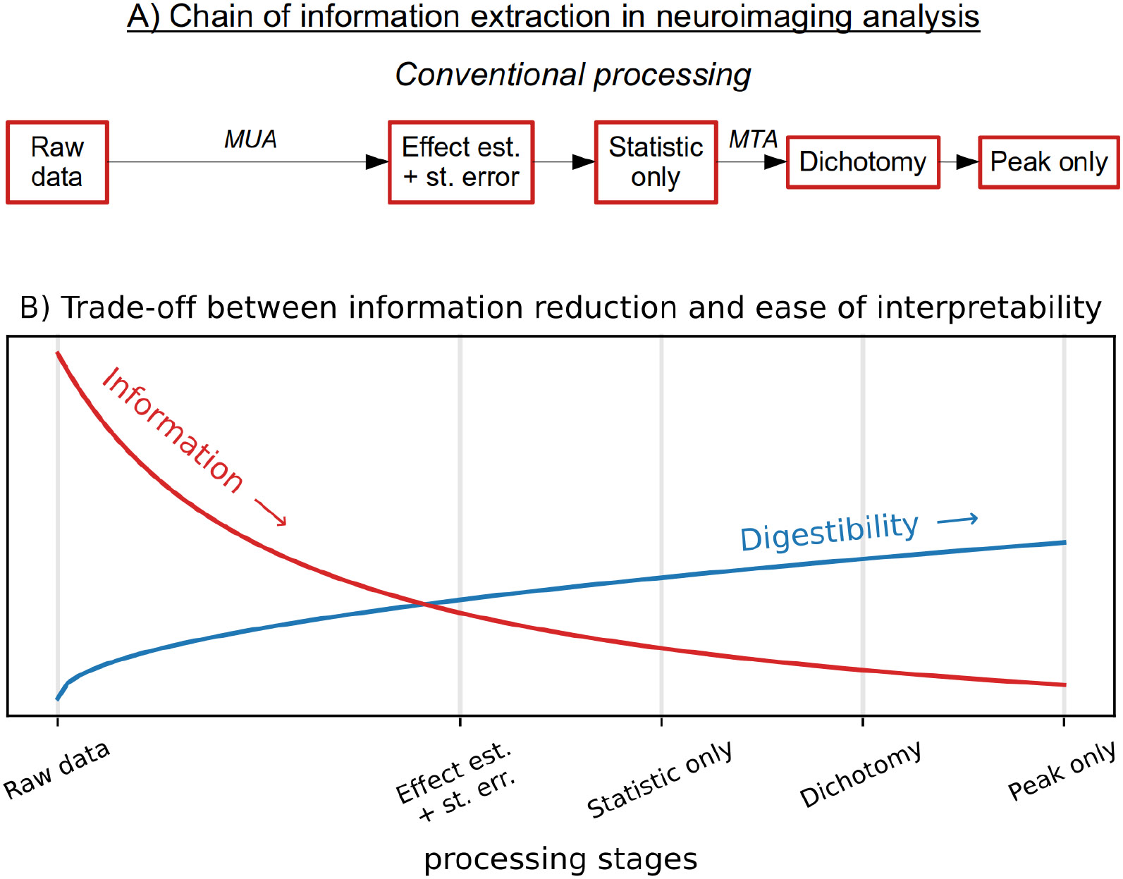
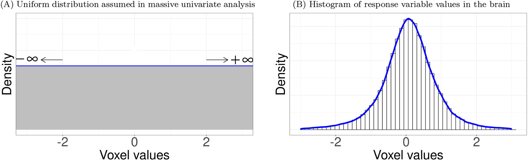
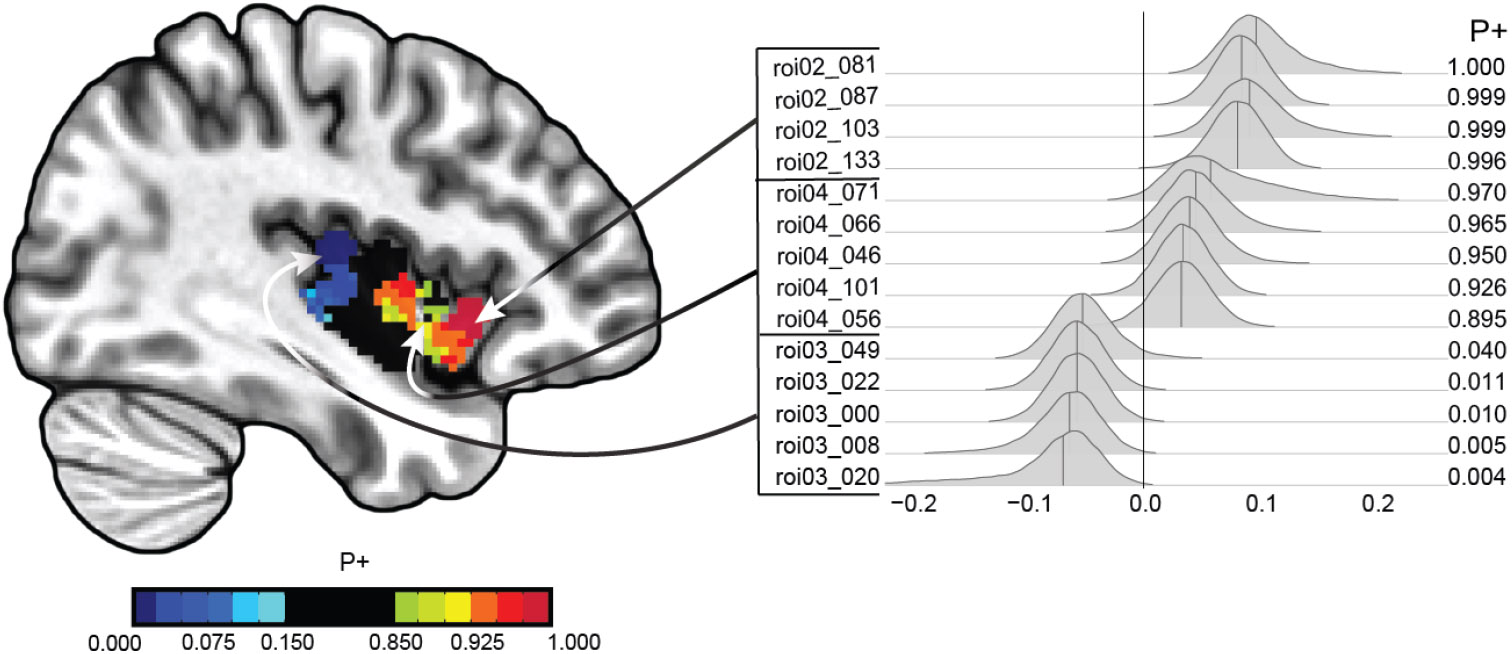
Neuroimaging relies on separate statistical inferences at tens of thousands of spatial locations. Such massively univariate analysis typically requires an adjustment for multiple testing in an attempt to maintain the family-wise error rate at a nominal level of 5%. First, we examine three sources of substantial information loss that are associated with the common practice under the massively univariate framework: (a) the hierarchical data structures (spatial units and trials) are not well maintained in the modeling process; (b) the adjustment for multiple testing leads to an artificial step of strict thresholding; (c) information is excessively reduced during both modeling and result reporting. These sources of information loss have far-reaching impacts on result interpretability as well as reproducibility in neuroimaging. Second, to improve inference efficiency, predictive accuracy, and generalizability, we propose a Bayesian multilevel modeling framework that closely characterizes the data hierarchies across spatial units and experimental trials. Rather than analyzing the data in a way that first creates multiplicity and then resorts to a post hoc solution to address them, we suggest directly incorporating the cross-space information into one single model under the Bayesian framework (so there is no multiplicity issue). Third, regardless of the modeling framework one adopts, we make four actionable suggestions to alleviate information waste and to improve reproducibility: 1) model data hierarchies, 2) quantify effects, 3) abandon strict dichotomization, and 4) report full results. We provide examples for all of these points using both demo and real studies, including the recent Neuroimaging Analysis Replication and Prediction Study (NARPS).

Keywords: Bayesian multilevel modeling; data hierarchy; dichotomization; effect magnitude; information waste; multiple testing problem; result reporting.


Figures

Figure 1:
Figure 1:
Statistical inferences in neuroimaging. (A) Schematic view of standard analysis: each voxel among tens of thousands of voxels is tested against the null hypothesis (voxel not drawn to scale). (B) Clusters of contiguous voxels with strong statistical evidence are adopted to address the multiple testing problem. (C) Full statistical evidence for an example dataset is shown without thresholding. (D) The statistical evidence in (C) is thresholded at voxelwise p = 0.001 and a cluster threshold of 20 voxels. The left inset shows the voxelwise statistical values from (C) while the right inset illustrates the surviving cluster. (E) The map of effect estimates that complements the statistical values in (C), providing percent signal change or other index of response strength, is shown. (F) For presenting results, we recommend showing the map of effect estimates, while using the statistical information for little or moderate thresholding (e.g., cluster threshold K = 20 voxels at voxelwise p = 0.05): “highlight” parts with strong statistical evidence, but do not “hide” the rest.
Figure 2:
Figure 2:
A schematic of conventional information extraction in neuroimaging. (A) The processing chain starts with raw data. Massively univariate analysis (MUA) produces a point estimate and its uncertainty (standard error) at every spatial unit. These are reduced to a single statistic map, which is then dichotomized using thresholding through multiple testing adjustment (MTA); finally, the analyst summarizes the regions based solely on their peak values, ignoring spatial extent. (B) The inherent trade-off between “information” and “digestibility” (y-axis has arbitrary units). While summarizing peak locations of dichotomized regions is a highly digestible form of output, this also entails a severe information loss. Here, we argue that providing effect estimates and standard errors, if possible, would be preferable, striking a better balance between information loss and interpretability.
Figure 3:
Figure 3:
Distributions of effects (“activation strength” in percent signal change) across space. (A) In massively univariate analysis, effects across all spatial units (voxels) are implicitly assumed to be drawn from a uniform distribution. Accordingly, the effect at each spatial unit can assume any value within (−∞, +∞) with equal likelihood. (B) Histogram of effect estimates (percent signal change) across 153,768 voxels in the brain from a particular study. Contrary to the assumption of uniform distribution implicitly made in massively univariate models, the effects approximately trace a Gaussian (or Student’s t) distribution.
Figure 4:
Figure 4:
Implications of dichotomization in conventional statistical practice. Case 1. What is the difference between a statistically significant result and one that does not cross a nominal threshold? Between the two hypothetical effects A and B that independently follow 𝒩(μ,σ2) (upper left: μA=0.2, σA=0.1 (blue); μB=0.4, σB=0.3 (red)), only A would be considered statistically significant. As the difference between the two random variables associated with A and B follows 𝒩(μBμA,σB2+σA2)=𝒩(0.2,0.1), it is not considered statistically significant (lower left: p = 0.26, area under the density of 𝒩(0.2,0.1) on the left side of the gray line x = 0), and effect B is mostly larger than A with a probability of 0.74 (lower left: area under the density of 𝒩(0.2,0.1) on the right side of the gray line x = 0). Case 2. How much information is lost due to the focus on binary statistical decisions? The two hypothetical effects A and C that independently follow 𝒩(μ,σ2)(upper right: μA=0.2, σA=0.1 (blue); μC=0.4, σC=0.2 (orange)) have the same p-values, and would be deemed indistinguishable in terms of statistical evidence alone. However, as the difference between the two random variables associated with A and C follows 𝒩(μCμA,σC2+σA2)=𝒩(0.2,0.05), C is mostly larger than A with a probability of 0.81 (lower right: area under the density of 𝒩(0.2,0.05) on the right side of the gray line x = 0). This comparison illustrates the information loss when the sole focus is on statistic or p value, which is further illustrated between the second and third blocks in Fig. 2.
Figure 5:
Figure 5:
Meta-analysis example. (A) Hypothetical results of 11 studies analyzing the same data (or 11 studies of the same task), with results summarized by the estimate of the effect, y^i (where i is the study index), and its standard error, σ^i. A total of 3/11 effects would be deemed statistically “significant” (red asterisks) according to standard cutoffs. From this perspective, one might say there is inconsistency or “considerable variability” of study results. (B) A different picture emerges if the same studies are combined in a meta-analysis: the overall evidence (area under the curve to the right of zero) points to a positive effect. The posterior distribution of the effect based on Bayesian multilevel modeling provides a richer summary of the results than (A). The shaded blue area indicates the 95% highest density interval (0.36, 0.83) surrounding the mode 0.63 (dashed blue line). (C) The individual results from (A) are presented (dots indicate y^i, horizontal lines show the uncertainty intervals of one standard error σ^i, and red asterisks mark the individually “significant” studies), along with the meta-analysis distribution information (colors as in B). With the full information present, we can evaluate the study consistency and overall effect more meaningfully.
Figure 6:
Figure 6:
Bayesian multilevel (BML) modeling at the region level. (A) Population-level analysis was performed with an FMRI study of 124 subjects. Each curve shows the posterior distribution (probability density). Colors represent values of P+: the posterior probability that the effect is positive. The analysis revealed that over one third of the regions exhibited considerable statistical evidence for a positive effect. In contrast, with massively univariate analysis, only two regions survived multiple testing adjustment. (B) The BML performance was assessed and compared to the conventional approach. Posterior predictive checks visually compare model predictions against raw data. The BML model generated a better fit to the data compared to the general linear model (GLM) used in the massively univariate analysis (MUA).
Figure 7:
Figure 7:
Bayesian multilevel voxelwise results. The right part of the figure illustrates posterior distributions of voxels from three subregions of the insula (voxels selected to illustrate some of the range of statistical evidence). Colors represent values of P+: the posterior probability that one condition (uncontrollable group) is greater than the other (controllable group). Values closer to 1 indicate stronger evidence that uncontrollable is greater than controllable, while values closer to 0 indicate the opposite (values computed based on the posterior distributions of the difference of the two conditions correspond to the tail areas of the posteriors). The computational time was about two weeks for this dataset with 126 subjects and approximately 1,000 voxels on a Linux server using 4 Markov chains.
Figure 8:
Figure 8:
Time series modeling and trial-based analysis. Consider an experiment with five face stimuli. (A) Hypothetical times series. (B) The conventional modeling approach assumes that all stimuli produce the same response, so one regressor is employed. (C) Condition-level effect (e.g., in percent signal change) is estimated through the regressor fit (green). (D-E) Trial-based modeling employs a separate regressor per stimulus, improving the fit (dashed blue). (F-G) Technically, the condition-level modeling allows inferences to be made at the level of the specific stimulus set utilized, whereas the trial-based approach allows generalization to a face category.
Figure 9:
Figure 9:
Trial-level versus condition-level modeling. Posterior distributions for the effect of reward (vs. control) cues for each region of interest. Although the two approaches provided comparable results, trial-level modeling (A) showed stronger evidence for left and right amygdala than the condition-level counterpart (B).
Figure 10:
Figure 10:
Comparison of FMRI information extraction for conventional and proposed Bayesian multilevel (BML) approaches (cf. Fig. 2). (A) The two approaches run parallel, but in the “proposed” first step BML puts data into a single model (removing the need for multiple testing adjustment later), and the information is partially pooled and shared across space. (B) The proposed multilevel framework produces an intermediate output of posterior distributions (lacking in the conventional approach) that carry rich information about parameter and model fitting. Partial pooling also improves model efficiency and avoid potential overfitting. This information advantage over the conventional method carries on to later stages. Thus, while the “digestibility” of results increases similarly at each stage, the drop-off in information content is slower in the proposed approach. The dotted part of the proposed steps reflects that we strongly suggest not including the steps that the traditional approaches at present perform, due to the wasteful information loss incurred.

Similar articles

Cited by

References

    1. Botvinik-Nezer R, Holzmeister F, Camerer CF, Dreber A, Huber J, Johannesson M, et al. Variability in the analysis of a single neuroimaging dataset by many teams. Nature. 2020. Jun;582(7810):84–8. - PMC - PubMed
    1. Zhang L, Guindani M, Versace F, Engelmann JM, Vannucci M. A spatiotemporal nonparametric Bayesian model of multi-subject fMRI data. Annals of Applied Statistics. 2016. Jun;10(2):638–66.
    1. Worsley KJ, Evans AC, Marrett S, Neelin P. A Three-Dimensional Statistical Analysis for CBF Activation Studies in Human Brain. Journal of Cerebral Blood Flow & Metabolism. 1992. Nov;12(6):900–18. - PubMed
    1. Forman SD, Cohen JD, Fitzgerald M, Eddy WF, Mintun MA, Noll DC. Improved Assessment of Significant Activation in Functional Magnetic Resonance Imaging (fMRI): Use of a Cluster-Size Threshold. Magnetic Resonance in Medicine. 1995;33(5):636–47. - PubMed
    1. Smith SM, Nichols TE. Threshold-free cluster enhancement: Addressing problems of smoothing, threshold dependence and localisation in cluster inference. NeuroImage. 2009. Jan;44(1):83–98. - PubMed

LinkOut - more resources