[Preprint]. 2025 May 29:arXiv:2505.23398v1.

Optimization and variability can coexist

Affiliations

Optimization and variability can coexist

Marianne Bauer et al. ArXiv. .

Abstract

Many biological systems perform close to their physical limits, but promoting this optimality to a general principle seems to require implausibly fine tuning of parameters. Using examples from a wide range of systems, we show that this intuition is wrong. Near an optimum, functional performance depends on parameters in a "sloppy" way, with some combinations of parameters being only weakly constrained. Absent any other constraints, this predicts that we should observe widely varying parameters, and we make this precise: the entropy in parameter space can be extensive even if performance on average is very close to optimal. This removes a major objection to optimization as a general principle, and rationalizes the observed variability.


Figures

FIG. 1:
FIG. 1:
Sampling the visual world. (a) A segment of the fly’s eye showing the regular lattice of lenses, which is echoed by a regular lattice of receptors and processing circuitry [25]. (b) Photoreceptor array in a human retina, with cells colored by their spectral sensitivity; note the more random arrangement [21]. (c) Array of N=1141 receptors on a regular lattice. (d) The same number of receptors scattered at random. (e) Functional performance—here, information per cell—from Eqs (5, 6), as a function of the signal–to–noise ratio for individual cells in the regular (blue) or random (red) arrangements. The range of SNR is chosen to match estimates for human cones in moderate daylight [26]. Inset shows the spectrum of eigenvalues of the Hessian of the functional performance, from Eq (2).
FIG. 2:
FIG. 2:
Optimizing the response to morphogens. (a) (left) Expression levels of Hb (red) and Kr (blue) as a function of position along the anterior–posterior axis of the embryo [33]. Solid lines are means over many embryos, and shaded regions show the standard deviation at each position. Expression of each gene is normalized so that 0g1, and position x is measured in units of the embryo length L. (right) An image of three “pair–rule” genes [37], whose expression depends on enhancers reading information from all gap genes and hence on the (hypothetical) compressed variable Z. (b) Discretizing combinations of expression levels. This is the optimal solution for ||Z||=10, with regions bounded by solid lines. Grey levels illustrate the probability density across all embryos and all positions. (c) Hessian matrices (insets), from Eq (2), and their eigenvalues for ||Z||=3 and ||Z||=10. The peak is normalized to 1.
FIG. 3:
FIG. 3:
Ion channel copy numbers in a small neural circuit. (a) Schematic of the core rhythm generating network in the crab stomatogastric ganglion [9], showing the anterior burster and pyloric dilator neurons (AB/PD), the lateral pyloric neuron (LP) and the pyloric neurons (PY), as well as their synaptic connections. (b) Voltage vs time for the three neurons, from the model described in Box 3. (c) Eigenvalues λ of the Hessian in Eq (2), where the functional performance is measured by the fractional closeness of the rhythm period (black) or duty cycle of the individual neurons (blue, green, yellow) and the parameters are the copy numbers of the different channel types in each cell.
FIG. 4:
FIG. 4:
A linear recurrent network of N=100 neurons. (a) Schematic network architecture (left). A network with internal connections Jij, is driven by a signal u(t) via an input weight vector m, and the output z(t) is a weighted sum of network activity via the readout weights n. Visualization of the network filter (right), from Eq (14). (b) Hessian eigenvalues λ of the cost function, Eq (16), for a random filter f*(τ) when perturbing the readout weights ni; different values of g in colors. (c) As in (B) when perturbing the recurrent connectivity weights Jij.
FIG. 5:
FIG. 5:
Eigenvalue spectrum of the Fisher information matrix for a network that learns the CIFAR–10 task. (a) Schematic of the network. (b) Performance of the network as function of time (“epoch”) during training. Training reaches a true optimum—zero loss—both for the natural task and for an artificial task in which the labels on images are randomized. (c) Eigenvalues of the Fisher information matrix F estimated from F˜ as in Eq (24). These estimates are based on n=1500 samples, probing the spectrum at different stages in the learning process. The distribution of eigenvalues converges as we increase n, especially in the tail of small eigenvalues.

References

    1. Rieke F. & Baylor D. A. Single photon detection by rod cells of the retina. Reviews of Modern Physics 70, 1027–1036 (1998).
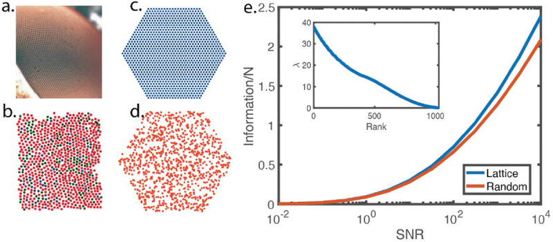
    1. Barlow H. B. The size of ommatidia in apposition eyes. Journal of Experimental Biology 29, 667–674 (1952).
    1. Snyder A. W. Acuity of compound eyes: Physical limitations and design. Journal of Comparative Physiology 116, 161–182 (1977).
    1. Berg H. C. & Purcell E. M. Physics of chemoreception. Biophysical Journal 20, 193–219 (1977). - PMC - PubMed
    1. Bialek W. Biophysics: Searching for Principles (Princeton University Press, Princeton NJ, 2012).

Publication types

LinkOut - more resources