Increasing mass spectrometry throughput using time-encoded sample multiplexing

Abstract

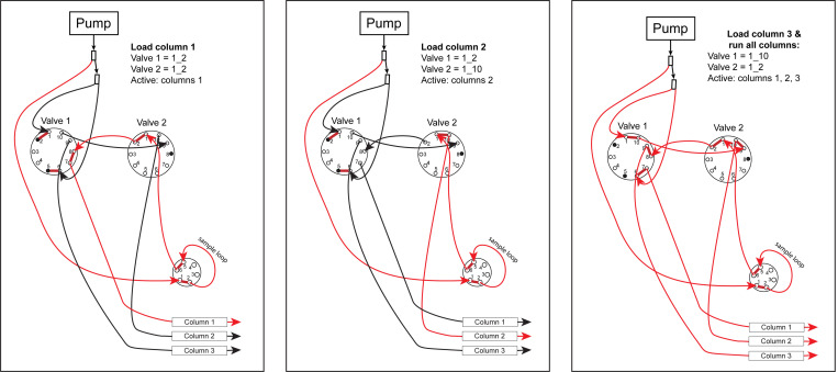
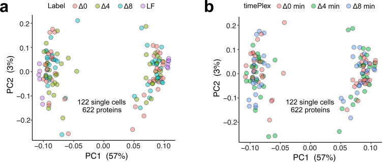
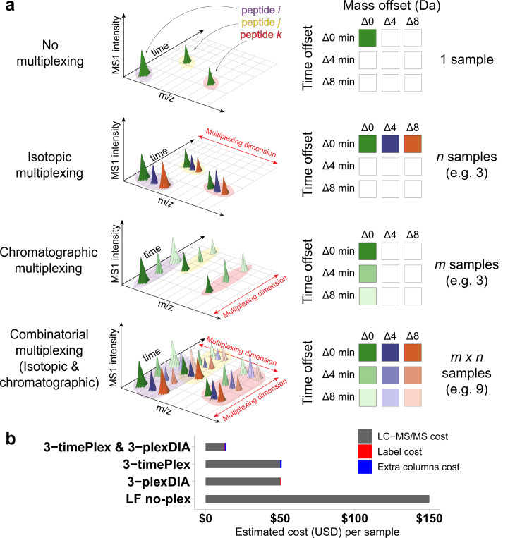
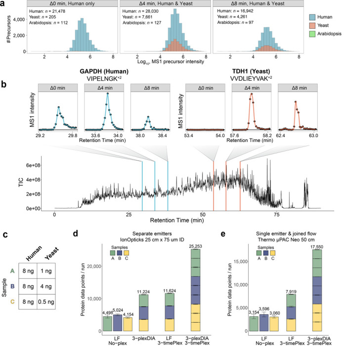
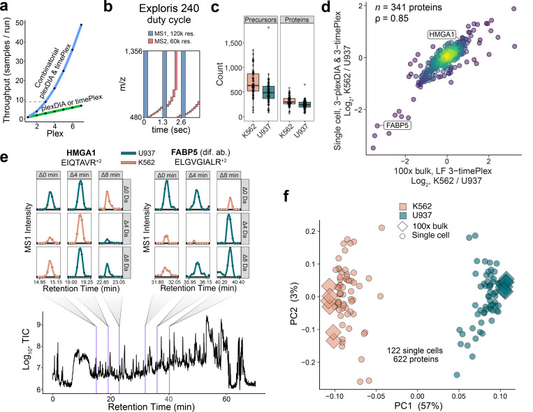
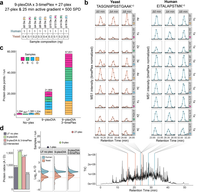
Liquid chromatography-mass spectrometry (LC-MS) can enable precise and accurate quantification of analytes at high-sensitivity, but the rate at which samples can be analyzed remains limiting. Throughput can be increased by multiplexing samples in the mass domain with plexDIA, yet multiplexing along one dimension will only linearly scale throughput with plex. To enable combinatorial-scaling of proteomics throughput, we developed a complementary multiplexing strategy in the time domain, termed 'timePlex'. timePlex staggers and overlaps the separation periods of individual samples. This strategy is orthogonal to isotopic multiplexing, which enables combinatorial multiplexing in mass and time domains when paired together, and thus multiplicatively increased throughput. We demonstrate this with 3-timePlex and 3-plexDIA, enabling the multiplexing of 9 samples per LC-MS run, and 3-timePlex and 9-plexDIA exceeding 500 samples / day with a combinatorial 27-plex. Crucially, timePlex supports sensitive analyses, including of single cells. These results establish timePlex as a methodology for label-free multiplexing and combinatorial scaling of the throughput of LC-MS proteomics. We project this combined approach will eventually enable an increase in throughput exceeding 1,000 samples / day.

Extended Data Fig. 1 |. Implementing 3-timePlex on Dionex UltiMate 3000 HPLC.

The diagram illustrates how samples are loaded sequentially for each column and then run together. Red indicates where net flow occurs. Flow is bifurcated from the NC pump, one line leads to the sample loop to push sample onto a given column, and the other line is bifurcated again to ports 1 and 6 of Valve 1. Plugs are utilized to maintain pressure to push sample through the loop during column loading. The valve-positions required to achieve this are noted on each panel of the diagram. Flow-rate of the methods are adjusted to account for the number of columns actively receiving flow. In this implementation, columns 1 and 2 are loaded at 300 nL/min, where only a single column is active a a time; this produces approximately 1.5x the backpressure as three columns run at 600 nL/min, which occurs during the ‘Load column 3 and run all columns’ phase.

Extended Data Fig. 2 |. Assessing carryover between timePlex channels Sample loading occurs through a shared sample-loop and transfer lines.

In some cases, this may result in unspecific binding of peptides onto these surfaces which will flow (unintended) into the third column during the active gradient. To mitigate this, samples were resuspended in 0.015% DDM for sample-loading. To assess the carryover, LF non-multiplexed data were searched as a 2-timePlex, attempting to quantify carryover (if any exists) in the unintended time channel. If signal was only detected in the intended time channel, that ratio was given a separable value of 1e-6 (green), if it was only detected in the unintended channel the ratio was given a value of 1e6 (blue), otherwise the observed ratio was plotted (red). Log10-transformed ratios reflect mostly missing data in the unintended time channel, and low signal for non-missing values. The median intensity of the non-missing data was 5.7% of the intensity of the intended time-channel.

Extended Data Fig. 3 |. Model architecture for predicting RTs

The model is a hybrid CNN and fully connected feedforward DNN which takes inputs of shape (30, 20), 30 being the peptide length and 20 being placeholders for each amino acid. There are 4 1D convolutional layers with kernel size = 4. The number of filters applied at each convolutional layer was set to double, starting at 32 and ending with 256. Max pooling = 2 was used for the final two layers. The final convolutional layer was flattened and fed into a fully connected feed-forward deep neural network with 1000, 256, 128, 64, and 32 nodes at each layer. Swish activation functions were used at all layers, with the exception of the final layer which was linear for computing the final RT output.

Extended Data Fig. 4 |. Setting RT tolerances

JMod searches benefit from thresholding on a tightly set RT range, so a peptide is only considered within a specific RT window and not throughout the run. This is especially important in timePlex, where peptides must be correctly associated to their sample origin. To set appropriate RT windows, we compute a cumulative distribution on the validation dataset, comparing the original library RTs with the fine-tuned RTs. We fit the cumulative distributions as Gaussian or exponential, and choose the fit that best matches the actual distribution, setting the RT threshold at the 95th percentile. a Fine-tuning is not necessary for data where the library has accurate RTs, as is the case here where the libraries were acquired shortly after the benchmarking runs and originate from the same columns used in the benchmarking data. b However, in cases where the library RTs do not properly model the empirical RTs, fine-tuning (orange) is highly beneficial, allowing for a smaller range to consider a peptide eluting. Here the library originates from RTs from IonOpticks columns, leading to a large discrepancy between what is empirically observed on μPAC columns (blue).

Extended Data Fig. 5 |. Investigating the effect of the 3 column separate emitter approach (background spray)

Here we investigate how the 3-column setup alone (not necessarily timePlex) impacts ion intensities and coverage relative to standard proteomics acquisition from a single emitter. The flow rate for the 3 column approach is 600 nL/min (approximately 200 nL/min/column) or 200 nL/min for a 1 column setup. a Ratio of precursor MS1 intenisites for the same samples acquired when 3 columns are spraying a total of 600 nL/min (however, only 1 column is actively separating a sample), or 1 column is spraying 200 nL/min. The 3-column setup results in approximately 2-fold lower MS1 intensities. The red dashed line indicates the median of the distribution. b We investigate how the 3-column setup impacts precursors identified for non-timePlex applications. The data reflect a 25% reduction in precursors identified with the 3-column setup, and c an approximately 20% reduction in protein coverage.

Extended Data Fig. 6 |. Spectral library quality becomes increasingly important at high-plex

a Triplicates of each plexDIA or combinatorial plexDIA & timePlex set were acquired, resulting in 9 runs for 3-plexDIA and 3 runs for 3×3 plexDIA & timePlex. Shown is the number of precursors identified for each run, searched with an unoptimized library (blue) or mTRAQ optimized library (red). b The same data, but shown as the change in the number of precursors identified as a result of searching data with an unoptimized library or mTRAQ optimized library. Searching data with an optimized spectral library results in a greater percentage increase of identifications at higher plex.

Extended Data Fig. 7 |. Investigating column-specific differences with timePlex

a Full width half max (FWHM) of precursor elutions was intersected across columns and implementations for the ‘separate emitters’ approach using IonOpticks 25cm x 75μm columns, or the ‘single emitter’ approach using μPAC Neo 50 cm columns, and plotted as density plots; a vertical black line marks the median of the distributions. b The ‘separate emitters’ approach using IonOpticks columns produced similar precursor coverage across columns. In the figure, each point represents a replicate and each facet corresponds to a samples (A, B, C). c Similar trends are observed for the ‘single-emitter joined flow’ approach using Thermo μPAC Neo columns, however the the 3rd column consistently under-performed the first two.

Extended Data Fig. 8 |. Precursor ratio counts between human and yeast benchmarking samples

a-c Number of precursor ratios quantified for each method between samples A/B, A/C, and B/C.

Extended Data Fig. 9 |. Investigating the presence of mass-tag and timePlex batch effects in PCA after batch correction

a PCA of single-cells and bulk samples colored by the mass tag label with which they were acquired. b PCA of single-cells and bulk samples colored by the timePlex channel with which they were acquired. This also corresponds to the LC column which was used.

Figure 1 |. Multiplexing in the time and mass domains is combinatorial

a Illustration of precursor elution curves for no multiplexing, plexDIA, timePlex, and combined timePlex & plexDIA data acquisitions. Combinatorial timePlex & plexDIA enables multiplicative scaling of the number of samples acquired / run. b Estimated cost for LC-MS/MS analysis per sample for different levels of multiplexing. The total cost per sample is estimated assuming $150/hr for LC-MS/MS, approximately $1k/column with an average 1,000-run lifespan, and the cost to label 1 μg of protein with commercially available mTRAQ (approximately $0.36).

Figure 2 |. Enabling timePlex analysis through accurate RT prediction

a Design showing two implementations of timePlex. The time-offsets are encoded through differences in the volumes of the transfer lines. b Conceptual illustration of repeated observations of peptides species systematically offset in time. c Illustration of RT predicting model. Peptide sequences were one-hot encoded and a hybrid convolutional neural network and deep neural network architecture was trained to predict retention times for label-free (LF) and mTRAQ-labeled peptides. Models were trained on 91,657 LF peptides or 56,645 mTRAQ-labeled peptides. d Test data, which were withheld from training, were used to evaluate the performance of the RT predictor. e To evaluate the model’s ability to fine-tune RT’s from new data, residuals were computed between the original RT predictions of the model (shown in blue), and after finetuning on approximately 3,200 peptides (shown in orange); the plotted data is the test-set withheld from fine-tuning. The 90th percentile boundaries are shown with orange and blue lines. f The original library iRTs predicted during DIANN in-silico library generation of LF data were used to visualize a typical starting point of RT accuracies, as shown in the left panel. For each run, our model is updated on the initial search results to fine-tune RTs to be used in the final search. The final search output is shown in the right panel with the library RTs for the middle timePlex channel. A precursor-set ([TRPVVAAGAVGLAQR]+3) is highlighted in pink to show it’s library RT before (left panel) and after (right panel) transfer learning.

Figure 3 |. Benchmarking timePlex protein coverage and throughput scalability

a LF 3-timePlex data was acquired for human only, human & yeast, and human & yeast samples present in Δ0 min, Δ4 min, and Δ8 min timePlex channels, respectively. The data was searched with a human, yeast, and arabidopsis spectral library. The number of precursor identifications is shown in each sub-panel for each species in addition to overlapping histograms of MS1 intensities for all precursors identified. At 1% FDR 21,478, 28,030, and 16,942 human precursors, 205, 7,661, and 4,261 yeast precursors, and 112, 127, and 97 arabidopsis precursors were identified in the three timePlexes. b The total ion chromatogram (TIC) of the missing-species run is displayed in addition to extracted ion chromatograms for a human GAPDH precursor and a yeast homolog of GAPDH (TDH1). The data show signal for human precursors across all three time-channels and a relative absence of yeast signal in the Δ0 min time-channel. c Sample composition for benchmarking protein coverage and quantitative accuracy. d Sample-specific proteins identified per run at 1% FDR for LF no-plex, 3-plexDIA, LF 3-timePlex, and 3-timePlex & 3-plexDIA with the ‘separate emitters’ approach. e Protein data points identified per run at 1% FDR for LF no-plex, LF 3-timePlex, and 3-timePlex & 3-plexDIA with the ‘single emitter & joined flow’ approach.

Figure 4 |. Benchmarking timePlex quantitative accuracy

a Correcting changes in the relative abundances of precursor intensities across the gradient. This change is systematic and correctable as shown in quantitative assessments before and after the correction was applied. The relative intensity panels correspond to a single timePlex channel in a single run, and the quantitative ratio panels compare that timePlex channel to another channel in that same run, in this case Sample B and C are shown for yeast (orange) and human (blue) precursors. All quantitation is from MS1 precursor intensities. b Distribution density plots for MS1 ratios of human and yeast precursors in common between samples B and C (n=9,884) are shown for both timePlex implementations to assess quantitative accuracy. Black horizontal lines mark the median of each respective distribution. c-e MS1 quantitation is shown for precursor ratios in common across all four methods and shown as scatter and box plots. The following abbreviations are used: LF-np: LF no-plex, 3-pD: 3-plexDIA, 3-tP: 3-timePlex, and 3×3: 3×3 plexDIA & timePlex. f Comparisons of MS1 and MS2-level quantitation are shown for precursor ratios in common across methods. The absolute-values of the errors between expected and observed fold-changes (FC) for each precursor ratio are shown as distributions with black vertical lines indicating the median.

Figure 5 |. Increasing the throughout of single-cell proteomics using combinatorial multiplexing with timePlex and plexDIA

a The throughput of combinatorial plexDIA and timePlex scales quadratically, while each individually scales linearly. The dashed red line marks the throughput achieved in this implementation of 3×3 plexDIA & timePlex. b All data was acquired on an Orbitrap Exploris 240. Here, the duty cycle is illustrated, which consisted of 12 MS2 scans of variable width and an MS1 scan scheduled every 1.3 seconds. c Single-cell data from Exploris 240 acquired with 3×3 plexDIA & timePlex identified a median of 631 and 486 precursors and 295 and 242 proteins per K562 and U937 cell, respectively. d Averaged fold-changes from single-cells of K562 and U937 cell lines agrees with bulk quantitation acquired by LF 3-timePlex (ρ=0.85). Highlighted is a protein, FABP5, found to be differentially abundant between the cell lines, and a highly abundant protein, HMGA1. e The raw MS1 extracted intensities from single-cells are plotted for a single 3×3 plexDIA & timePlex run, for precursors corresponding to HMGA1 and FABP5. The differential abundance of FABP5 is observed in the raw data of MS1 XICs, where it is higher on average in U937 cells. f PCA was performed on the subset of proteins quantified both in the bulk and single-cell samples. The bulk (diamond) and single-cell (circle) data points show agreement in their cell-type specific separation along PC1.

Figure 6 |. Combining 9-plexDIA with 3-timePlex increases proteomics throughput 27-fold

a Proteomic compositions of samples A-D consisted of 1 ng human digest and variable amounts of mixed yeast digest (0.1–0.4 ng). These samples were labeled with PSMtags and pooled to enable 9-plexDIA. Samples were acquired at a rate exceeding 500 samples/day with combinatorial 9×3 plexDIA & timePlex. b Extracted ion chromatograms for yeast and human precursors from the 9×3 plexDIA & timePlex data. c Number of sample-specific proteins identified per run at 1% FDR for label-free no-plex, 9-plexDIA, and 9-plexDIA and 3-timePlex. d Bar plots show the number of protein ratios quantified across triplicates for LF no plex, 9-plexDIA, and 9×3 plexDIA & timePlex. The intersecting proteins across methods was used to benchmark quantitative accuracy at MS2-level, shown as density plots of the measured protein ratios.

References

1. Demichev V. et al. dia-PASEF data analysis using FragPipe and DIA-NN for deep proteomics of low sample amounts. en. Nature Communications 13, 3944. (2024) (July 2022). - PMC - PubMed
1. Kreimer S. et al. Parallelization with Dual-Trap Single-Column Configuration Maximizes Throughput of Proteomic Analysis. Analytical chemistry 94, 12452–12460 (Sept. 2022). - PMC - PubMed
1. Xie X. et al. Multicolumn Nanoflow Liquid Chromatography with Accelerated Offline Gradient Generation for Robust and Sensitive Single-Cell Proteome Profiling. Analytical Chemistry 96, 10534–10542 (July 2024). - PMC - PubMed
1. Nagae N., Itoh H., Nimura N., Kinoshita T. & Takeuchi T. Rapid separation of proteins and peptides by reversed-phase microcolumn liquid chromatography. Journal of Microcolumn Separations 3, 5–9 (1991).
1. Moritz R. L. & Simpson R. J. Purification of proteins and peptides for sequence analysis using microcolumn liquid chromatography. Journal of Microcolumn Separations 4, 485–489 (1992).
Publication types
LinkOut - more resources