Uncertainty-aware traction force microscopy

Abstract

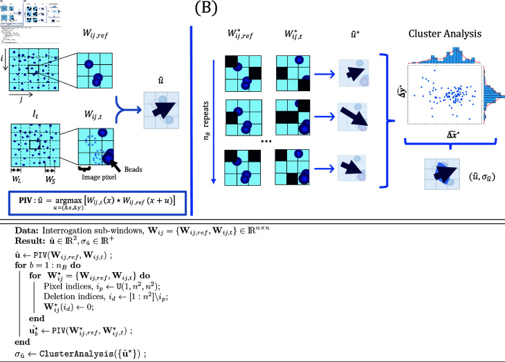
Traction Force Microscopy (TFM) is a versatile tool to quantify cell-exerted forces by imaging and tracking fiduciary markers embedded in elastic substrates. The computations involved in TFM are often ill-conditioned, and data smoothing or regularization is required to avoid overfitting the noise in the tracked displacements. Most TFM calculations depend critically on the heuristic selection of regularization (hyper-) parameters affecting the balance between overfitting and smoothing. However, TFM methods rarely estimate or account for measurement errors in substrate deformation to adjust the regularization level accordingly. Moreover, there is a lack of tools for uncertainty quantification (UQ) to understand how these errors propagate to the recovered traction stresses. These limitations make it difficult to interpret the TFM readouts and hinder comparing different experiments. This manuscript presents an uncertainty-aware TFM technique that estimates the variability in the magnitude and direction of the traction stress vector recovered at each point in space and time of each experiment. In this technique, a non-parametric bootstrap method perturbs the cross-correlation functional of Particle Image Velocimetry (PIV) to assess the uncertainty of the measured deformation. This information is passed on to a hierarchical Bayesian TFM framework with spatially adaptive regularization that propagates the uncertainty to the traction stress readouts (TFM-UQ). We evaluate TFM-UQ using synthetic datasets with prescribed image quality variations and demonstrate its application to experimental datasets. These studies show that TFM-UQ bypasses the need for subjective regularization parameter selection and locally adapts smoothing, outperforming traditional regularization methods. They also illustrate how uncertainty-aware TFM tools can be used to objectively choose key image analysis parameters like PIV window size. We anticipate that these tools will allow for decoupling biological heterogeneity from measurement variability and facilitate automating the analysis of large datasets by parameter-free, input data-based regularization.

Fig 1. TFM-UQ method improves traction stress inference and provides uncertainty bounds.

(A) Traction Force Microscopy experiment. Reference image $({\mathit{I}}_{ref})$ of the substrate markers is obtained at a stress-free state. Session image(s) $({\mathit{I}}_t)$ of the substrate marker are obtained at the time point of interest. (B) Existing TFM workflow provides a point estimate of forces but does not consider the variability in the traction stress due to the microscopy images and TFM implementation. (C) The proposed TFM-UQ method considers the local image quality, ambiguity in regularization parameter selection, and the numerical implementation to provide locally adaptive smoothing and error bars.

Fig 2. Particle Image Velocimetry with Uncertainty Quantification (PIV-UQ) method.

Top: Schematic of PIV and PIV-UQ. (A) The image data $\mathit{I}$ is sectioned into overlapping square sub-windows ${\mathbf{W}}_{ij}$ of length W_L (n² pixels), their centers separated by W_S. PIV computes the most likely displacement for each sub-window ${\mathbf{W}}_{ij}$ that corresponds to the maximum of the cross-correlation metric. Each pixel of ${\mathbf{W}}_{ij}$ contributes to the correlation value, hence the maximization procedure. (B) PIV-UQ method bootstraps the contribution of individual pixels to the cross-correlation metric. Pixel indices are randomly sampled with replacement and the unsampled indices are set to 0 (Black pixels). Backslash denotes the set difference operation and $\mathtt{\text{U}}(1,n^2,n^2)$ represents uniformly distributed n² samples in the interval [1,n²]. The bootstrapped sample of size n_B is analyzed for multiple possible clusters and outliers, subsequently providing a metric of variability for each sub-window (i.e., for each discrete vector of the deformation field). Bottom: PIV-UQ bootstrap algorithm.

Fig 3. Hierarchical Bayesian TFM formulation for adaptive and self-consistent regularization.

The problem of choosing a regularization parameter is treated in a Bayesian formulation. Substrate deformation (${\mathit{u}}_{\text{h}}$) is the observed quantity, and it is modeled as the additive contribution of traction stresses ($\mathit{t}$), locally resolved PIV measurement uncertainty ${\mathit{\Sigma }}_{\text{PIV}}$ and a global model error $(\beta )$ that is unknown. The hierarchical formulation allows to express unknown hyper-parameters ($\alpha ,\beta )$ for the prior on traction stress field and the model error term as random variables to be inferred. Therefore, a non-informative hyper-prior (${\varphi }_s$) is specified to the hyper-parameters. The priors can encode reasonable assumptions such as smoothness and global force balance. Markov Chain Monte Carlo (MCMC), specifically an hybrid Gibbs sampling, is used for inference from the marginal posterior distribution, $p(\mathit{t}|{\mathit{u}}_{\text{h}})$.

Fig 4. Hybrid Gibbs sampler for TFM UQ inference.

Fig 5. PIV-UQ synthetic validation.

(A, D) Gaussian profile synthetic beads are randomly generated at varying signal-to-noise ratio (SNR) of image pixel noise. A uniform (U) displacement field (B, E) or a shear (S) displacement field (C, F) is applied to the synthetic beads and PIV-UQ is performed as described in § 2.2. In (B,C,E and F), left columns show ground-truth data consisting of applied displacement field vectors overlaid on contour maps of ensemble standard deviation (${\mathit{u}}_{ens}$ and ${\sigma }_{u,ens}$). The right columns represent the same data estimated from PIV-UQ, ${\mathit{u}}_{PIV}$ and ${\sigma }_{u,PIV}$. Units are in pixels (px). (G) Joint distribution of $({\sigma }_{u,ens},{\sigma }_{u,PIV})$ for uniform (U) and shear (S) deformation fields for W_L of 32 and 64 px. Analysis procedure is described in Fig A in S1 Text (H) RMS of ensemble standard deviation and PIV UQ bootstrap estimates are compared for varying SNR values. (I) PIV Window size as a function of SNR with ${\sigma }_{u,\text{PIV}}$ isolines derived from data presented in (H). N = 50 realizations of $1024\times 1024$ pixels images were generated.

Fig 6. Synthetic pipeline to simulate experimentally relevant, spatially heterogeneous noise levels in TFM.

(A) Synthetic traction stress generated from four traction islands of Gaussian profile, ${\mathit{t}}_G$, one in each quadrant with a maximum stress of $500\text{Pa}$. (B) Synthetic displacement field resulting from the traction profile in (A). Substrate of $E=5$ KPa and Poisson’s ratio of 0.45 is used here. (C) Schematic depicting spatially heterogeneous noise addition directly to the synthetic image by varying fluorescent bead density in X-direction. The synthetic image also has image pixel noise equivalent to SNR  = 50 (D) Synthetic fluorescent bead image encoding image pixel noise and bead density variations. (E) PIV-UQ deformation measurement ${\mathit{u}}_{\text{PIV}}$ of the simulated bead images (D). (F) PIV-UQ estimation of uncertainty (standard deviation ${\sigma }_{u,\text{PIV}}$) showing higher uncertainty increasing with x-direction in agreement with noise addition process (C).

Fig 7. TFM-UQ adaptively regularizes based on the local displacement uncertainty.

(A) Mean marginal posterior traction stress distribution ($\hat{\mathbf{t}}=𝔼[\mathit{t}|{\mathit{u}}_{\text{h}}]$) approximated from Hybrid-Gibbs sampling. (Based on synthetic data described in Fig 6A.) (B) Pointwise marginal posterior uncertainty (standard deviation ${\sigma }_t$) of posterior traction stress (C) L-curve to determine Tikhonov regularization parameter $\lambda$ in traditional TFM methods. ${\lambda }_L$ and ${\lambda }_H$ are regularization parameters obtained from L-curve corners of homoskedastic synthetic simulations with spatially uniform low noise (L) or high noise (H). (D, E, F) Tikhonov regularized traction stress field corresponding to L-curve corner ${\lambda }_D$, low noise ${\lambda }_L$ and high noise ${\lambda }_H$ respectively. $\mathbf{L}$ is the discretized Laplacian operator. (G, H, I) Tikhonov regularized traction stress field, with $\mathbf{L}=\mathbf{U}$ identity matrix. ${\lambda }_D$,${\lambda }_L$ and ${\lambda }_H$ were determined to match 95^th percentile of traction stress magnitude with the respective fields in (D-F).

Fig 8. TFM-UQ captures variability associated with microscopy image quality.

(A) Brightfield image of C3H/10T1/2 cell cultured on fibronectin micropatterned island of length $75\mu \text{m}$ (Red dashed outline). (B) “Raw” wide-field fluorescent bead image (beads of size $0.2\mu \text{m}$). (C) “BGS” Background subtracted image processed from (B). (D, G, J) ${\mathit{u}}_{\text{PIV}}$ (arrows) overlaid on PIV-UQ uncertainty field (${\sigma }_{u,\text{PIV}}$) corresponding to raw WL-128, BGS WL-128 and BGS WL-64 respectively. Here, WL denotes the PIV interrogation window size W_L. (E, H, K) Mean marginal posterior traction stress field ($\hat{\mathbf{t}}$) corresponding to Raw WL-128, BGS WL-128 and BGS WL-64 respectively. (F, I, L) Traction stress signal-to-noise ratio ($SN{R}_{\mathit{t}}$) plotted as a heatmap corresponding to Raw WL-128, BGS WL-128 and BGS WL-64 respectively. Overlaid uncertainty arrows denote the pointwise angular uncertainty corresponding to 1 circular std. dev. of marginal posterior $p(\mathit{t}|{\mathit{u}}_{\text{h}})$. Scale bar: $25\mu \text{m}$.

Fig 9. TFM-UQ applied to endothelial monolayer experiment demonstrates uncertainty propagation.

(A) Membrane labeling of HUVEC monolayers with CellMask. (B) Corresponding fluorescent bead image (beads of size $0.2\mu \text{m}$). Arrows indicate bead-related image artifacts (C) PIV-UQ displacement field ${\mathit{u}}_{\text{PIV}}$ (D) PIV-UQ uncertainty map, ${\sigma }_{u,PIV}$. White regions indicate “bad” PIV windows that were deleted and replaced as described in § 2.2. Uncertainty arrows denote the pointwise angular uncertainty corresponding to 1 circular std. dev. of bootstrapped PIV-UQ distribution. (E) Inferred mean marginal posterior traction stress, $\hat{\mathbf{t}}$ (F) Marginal posterior traction stress uncertainty field (${\sigma }_t$). Uncertainty arrows denote the pointwise angular uncertainty corresponding to 1 circular std. dev. of marginal posterior $p(\mathit{t}|{\mathit{u}}_{\text{h}})$. Scale bar : $25\mu \text{m}$

References

1. Harris AK, Wild P, Stopak D. Silicone rubber substrata: a new wrinkle in the study of cell locomotion. Science. 1980;208(4440):177–9. doi: 10.1126/science.6987736 - DOI - PubMed
1. Eyckmans J, Boudou T, Yu X, Chen CS. A hitchhiker’s guide to mechanobiology. Dev Cell. 2011;21(1):35–47. doi: 10.1016/j.devcel.2011.06.015 - DOI - PMC - PubMed
1. Hansen PC, O’Leary DP. The use of the L-curve in the regularization of discrete ill-posed problems. SIAM J Sci Comput. 1993;14(6):1487–503. doi: 10.1137/0914086 - DOI
1. Gómez-González M, Latorre E, Arroyo M, Trepat X. Measuring mechanical stress in living tissues. Nat Rev Phys. 2020;2(6):300–17. doi: 10.1038/s42254-020-0184-6 - DOI - PMC - PubMed
1. Kumar A, Placone JK, Engler AJ. Understanding the extracellular forces that determine cell fate and maintenance. Development. 2017;144(23):4261–70. doi: 10.1242/dev.158469 - DOI - PMC - PubMed
LinkOut - more resources