Forward modelling low-spectral-resolution Cassini/CIRS observations of Titan

Abstract

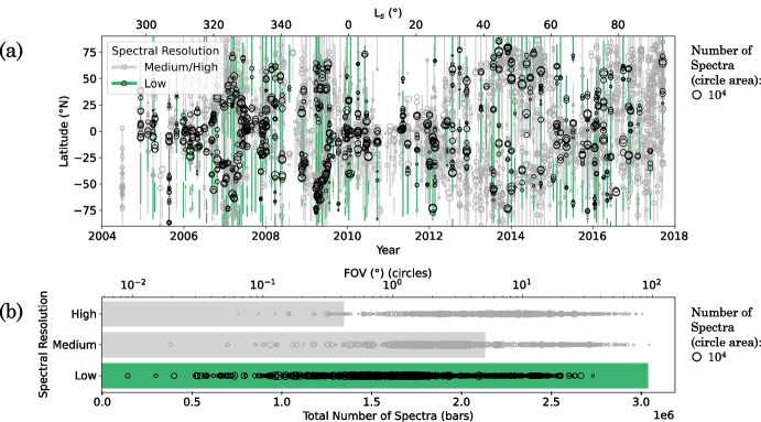
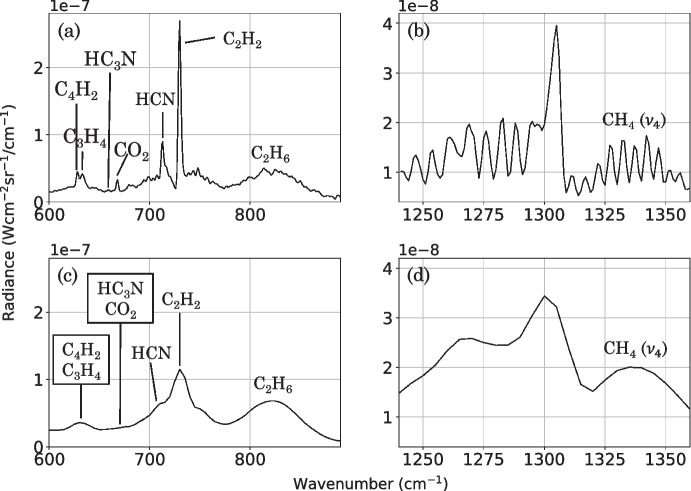
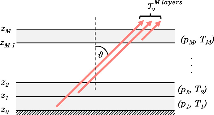
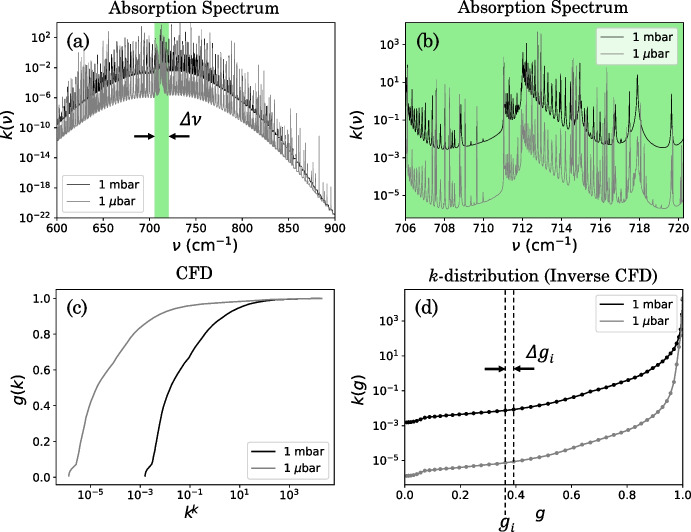
The Composite InfraRed Spectrometer (CIRS) instrument onboard the Cassini spacecraft performed 8.4 million spectral observations of Titan at resolutions between 0.5-15.5 cm^-1. More than 3 million of these were acquired at a low spectral resolution (SR) (13.5-15.5 cm^-1), which have excellent spatial and temporal coverage in addition to the highest spatial resolution and lowest noise per spectrum of any of the CIRS observations. Despite this, the CIRS low-SR dataset is currently underused for atmospheric composition analysis, as spectral features are often blended and subtle compared to those in higher SR observations. The vast size of the dataset also poses a challenge as an efficient forward model is required to fully exploit these observations. Here, we show that the CIRS FP3/4 nadir low-SR observations of Titan can be accurately forward modelled using a computationally efficient correlated- $k$ method. We quantify wavenumber-dependent forward modelling errors, with mean 0.723 nW cm ${}^{-2}$ sr^-1/cm^-1 (FP3: 600-890 cm^-1) and 0.248 nW cm ${}^{-2}$ sr ${}^{-1}$ / cm^-1 (FP4: 1240-1360 cm^-1), that can be used to improve the rigour of future retrievals. Alternatively, in cases where more accuracy is required, we show observations can be forward modelled using an optimised line-by-line method, significantly reducing computation time.

Keywords: Infrared spectroscopy(2285); Radiative transfer(1335); Titan(2186).

Fig. 1

Mission coverage of all CIRS nadir observations of Titan, with low-spectral resolution (SR) observations highlighted in green. a: Latitude coverage (bars) and mean latitude (circles) of each observation at the time of observation. b: Total number of spectra (shaded regions) acquired by CIRS at high (FWHM $\sim$ 0.5 cm^-1), medium (FWHM $\sim$ 2.5 cm^-1), and low (FWHM $\sim$ 14.5 cm^-1) SR, and field of view (FOV) (circles) of each observation. Circle area is proportional to the number of spectra in that observation. A circle area corresponding to ${10}^4$ spectra is shown for scale. Smaller FOV corresponds to higher spatial resolution. A large proportion of CIRS spectra have a low SR, and low-SR observations have good spatial and temporal coverage throughout the mission (2004–2017). Low-SR observations typically have a smaller FOV size and hence a higher spatial resolution

Fig. 2

Example CIRS FP3/4 measured Titan spectrum at a medium SR (FWHM = 2.5 cm^-1) (a, b) and a low SR (FWHM = 14.5 cm^-1) (c, d). Emission peaks of key gases in Titan’s atmosphere are labelled. A typical noise on an individual spectrum observed at a low-SR ($\sim 2.5$ nW cm${}^{-3}$sr${}^{-1}$/ cm^-1 for FP3 and $\sim 0.5$ nW cm${}^{-3}$sr${}^{-1}$/ cm^-1 for FP4) is less than on an individual spectrum observed at a medium-SR ($\sim 8$ nW cm${}^{-3}$sr${}^{-1}$/ cm^-1 for FP3 and $\sim 1.5$ nW cm${}^{-3}$sr${}^{-1}$/ cm^-1 for FP4). In the low-SR measured spectra, HCN, C₂H₂, C₂H₆, and CH₄ peaks are distinct, but C₄H₂ and C₃H₄ peaks are blended. HC₃N and CO₂ peaks are also blended

Fig. 3

An atmosphere can be modelled as M homogeneous layers, each of a constant pressure, $p_i$, and temperature, $T_j$. Observing along some path through an atmosphere, at zenith angle $\theta$, the transmission at the top of the atmosphere, ${\mathcal{T}}_{\nu }^{Mlayers}$, can be found by summing contributions from each homogeneous layer. Emission of radiation, along the viewing path, from each atmospheric layer is represented by red arrows

Fig. 4

Example Lorentz- and Doppler-broadened spectral line widths for some spectrally active gases in Titan’s atmosphere. The Lorentz line width (dashed lines) is due to collisions between molecules, and is dependent on atmospheric temperature and pressure. The Doppler line width (solid lines) is due to the relative velocity of a molecule with respect to the observer, and is dependent on atmospheric temperature. Typical values based on line data from HITRAN and GEISA. Line widths are shown at three latitude end members: 75^∘N (blue), 0^∘N (orange), and -75^∘N (purple) in Titan northern mid-winter (year 2005). Representative temperature profiles are taken from Teanby et al. [25] (Supplementary Material S3). The narrowest HWHM line width is approximately $4\times {10}^{-4}$ cm^-1 (C₆H₆). Hence, in a LBL forward model, a grid spacing of gs = $2\sqrt{2ln2}(4\times {10}^{-4}$ cm${}^{-1})\approx 9.4\times {10}^{-4}$ cm^-1 is required to Nyquist sample the minimum line width

Fig. 5

Convolution of an example LBL infinite resolution synthetic spectrum with an instrument function to produce a finite resolution spectrum. The spectrum emitted by an atmosphere has an infinite resolution. In observing the emission, the spectrum is smoothed by the finite-resolution viewing instrument. The resulting observed spectrum can be calculated by convolution of the infinite resolution spectrum with the viewing instrument’s apodisation function. The Hamming function is shown here as an example instrument function

Fig. 6

Comparison of synthetic Titan spectra produced with a line-by-line (LBL) forward model at varied underlying spectral grid spacing. a, b: Synthetic CIRS FP3 (a) and FP4 (b) Titan spectra computed with a LBL forward model are shown at three grid spacing end members – fine ($gs=2\times {10}^{-4}$ cm^-1, the gold-standard grid spacing which Nyquist samples the narrowest spectral line, solid line), coarse ($gs=1\times {10}^{-1}$ cm^-1, dashed line) and an optimal ($gs=9\times {10}^{-4}$ cm^-1 for FP3 and $gs=10\times {10}^{-4}$ cm^-1 for FP4, dotted line) grid spacing. c, d: FP3 (c) and FP4 (d) synthetic spectra computed with each underlying grid spacing are subtracted from the gold-standard synthetic spectrum. The maximum (max, diamonds) and root-mean-squared (RMS, circles) absolute radiance difference between the spectra are shown at three latitude end-members: 75^∘N (blue), 0^∘N (orange), and -75^∘N (purple) in Titan northern mid-winter (year 2005). A typical run-time to compute one synthetic Titan CIRS FP3/4 spectrum at each coarse grid spacing is also shown (coloured dashed lines). Representative NESR levels (2.5 nW cm${}^{-3}$sr${}^{-1}$/ cm^-1 for FP3, 0.5 nW cm${}^{-3}$sr${}^{-1}$/ cm^-1 for FP4, taken from Flasar et al. [8]) are labelled (grey dashed lines), including the limiting noise NESR/$\sqrt{4000}$. CIRS FP3/4 Titan nadir spectra can be forward modelled within the limiting noise level using a grid spacing less than the width of the narrowest spectral line in the FP3/4 region

Fig. 7

An example HCN absorption spectrum and k-distribution at two example altitudes in Titan’s atmosphere. a: A HCN absorption spectrum in the CIRS FP3 spectral range. b: The same spectrum but zoomed to a smaller spectral interval, with width equal to the average FWHM of CIRS low-spectral resolution (SR) observations ($\mathrm{\Delta }\nu =$ 14.25 cm^-1). This region is highlighted in green in a. c: Cumulative frequency distribution (CFD) of the absorption spectrum. d: The CFD is inverted to obtain a k-distribution. The k-distribution is sampled at NG g-ordinates following a Gaussian quadrature scheme. Ordinates are shown as circular points in d, where $NG=$ 50 in this example. Each is shown at two example altitudes in Titan’s atmosphere: 1 mbar (150 K, black line) and 1 $\mu$bar (170 K, grey line). The absorption spectrum (a) varies rapidly with wavenumber, whereas the k-distribution (d) is a smooth function in g-space which allows for coarser sampling and hence a computationally quicker forward model

Fig. 8

The two instrument functions used in different correlated-k (c-k) forward models. The first uses k-tables that model a square instrument function and the resulting spectrum is convolved with another square function to overall model a triangle instrument function (a). The second uses k-tables that model a Hamming instrument function and does not apply a second convolution in the forward model (b). The CIRS apodisation function is a Hamming function [8], that is often approximated as a triangle function for high-SR CIRS observations

Fig. 9

Comparison of the correlated-k (c-k) to the line-by-line (LBL) forward model. a, b: Synthetic CIRS FP3 (a) and FP4 (b) Titan spectra produced using a LBL forward model with a fine underlying spectral grid spacing ($gs=2\times {10}^{-4}$ cm^-1) (solid line), and using a c-k forward model with k-tables produced with a Hamming instrument (dotted line). Each is performed at three latitude end members: 75^∘N (blue), 0^∘N (orange), -75^∘N (purple) in Titan northern mid-winter (year 2005), assuming a 0^∘ emission angle. Representative temperature profiles are taken from Teanby et al. [25] (Supplementary Material S3). c, d: LBL-modelled spectra subtracted from c-k-modelled spectra. A typical measurement error is shown for comparison (blue shaded region). e–h: The same comparison as in a–d but at an emission angle of 60^∘. Spectra produced using a c-k forward model with Hamming k-tables are mostly consistent with the LBL spectra within the measured error

Fig. 10

Comparison of synthetic Titan spectra forward modelled using a correlated-k (c-k) method with Hamming k-tables sampled at NG = 50 and NG = 200 ordinates in cumulative-frequency-space (g-space). a, b: Synthetic CIRS FP3/4 Titan spectra produced using a line-by-line (LBL) and a c-k forward model. c, d: Radiance difference between the c-k and LBL-forward modelled spectra. Shown at three latitude end members: 75^∘N (blue), 0^∘N (orange), -75^∘N (purple) in Titan northern mid-winter (year 2005). A typical CIRS measurement error is shown (c, d, blue shaded region). A c-k forward model typically requires $\sim 30$ seconds (FP3) and $\sim 10$ seconds (FP4) for NG = 50 and $\sim 140$ seconds (FP3) and $\sim 40$ seconds (FP4) for NG = 200, wheras we find the LBL requires an average of 115 minutes (FP3) and 36 minutes (FP4) at optimal grid spacing

Fig. 11

Synthetic retrieval test of the correlated-k (c-k) forward model. a: Synthetic FP4 Titan spectra were produced using a gold-standard ($gs=2\times {10}^{-4}$ cm^-1) LBL forward model (solid lines), and a Gaussian noise was added at the minimum FP4 noise level. The FP4 spectra were fitted using a c-k forward model with Hamming k-tables (dotted lines), to retrieve atmospheric temperature (b). b: The retrieved temperature profile error envelopes (shaded regions) are consistent with the input temperature profiles (solid lines). The test was performed at three latitude end members: 75^∘N (blue), 0^∘N (orange), and -75^∘N (purple) in 2005, assuming a 0^∘ emission angle. c and d show the same as a and b, but assuming an emission angle of 60^∘

Fig. 12

Example Titan temperature and gas volume mixing ratio (VMR) profiles during Titan northern mid-winter (2005). a: Spatial coverage of the CIRS FP3 and FP4 focal planes during an example Titan observation (CIRS$\_013$TI$\_$FIRNADMAP$002\_$PRIME) on a Titan sphere. The centre of each 2^∘ latitude bin is plotted (red dots). Lines of constant latitude (blue, solid) and longitude (blue, dashed) are shown. The position of the sub-spacecraft point is indicated with a green dot. This observation was acquired at a spectral resolution of FWHM = 14.45 cm^-1. b: Number of spectra averaged over in each latitude bin, shown for FP3 as an example. Latitude bins have a width of 2^∘ and are spaced by 1^∘. c: Example retrieved (‘r’) vertical temperature profile [25] (solid line) and retrieved error (shaded area) at three latitude end members: 50^∘N (blue), 0^∘N (orange), and -50^∘N (purple). The temperature profile measured (‘m’) by the Huygens Atmospheric Structure Instrument (HASI) at approximately -10^∘N is also shown (black). d–i: VMR vertical profiles for some trace gases in Titan’s atmosphere at the same three latitudes in 2005. Gas vertical profiles are estimated by first assuming a VMR uniform with pressure then applying a condensation level, based on the retrieved temperature profile at that time and latitude. We assume that the VMR does not increase again at higher altitudes as the temperature increases

Fig. 13

Fits to low-spectral-resolution (SR) CIRS measured Titan spectra (observation CIRS$\_013$TI$\_$FIRNADMAP$002\_$PRIME acquired at FWHM = 14.45 cm^-1 on 22/08/2005). The retrieval was performed using a correlated-k (c-k) forward model with k-tables produced with the Hamming instrument function. Fitted (solid line) and measured (shaded region) FP3 (a) and FP4 (b) spectra are shown at three example latitudes: 50^∘N (blue), 0^∘N (orange) and -50^∘N (purple). The sub-spacecraft point is within 10^∘ of the equator during this observation. We use our estimated maximum average forward modelling errors, given in Appendix A. The goodness of fit, ${\chi }^2/n_y$, of each spectrum is labelled

References

1. Achterberg, R.K., Gierasch, P.J., Conrath, B.J., et al.: Temporal variations of Titan’s middle-atmospheric temperatures from 2004 to 2009 observed by Cassini/CIRS. Icarus 211(1), 686–698 (2011). 10.1016/j.icarus.2010.08.009. https://linkinghub.elsevier.com/retrieve/pii/S0019103510003155
1. Barth, E.: Microphysical modeling of ethane ice clouds in titan’s atmosphere. Icarus 162(1), 94–113 (2003). 10.1016/S0019-1035(02)00067-2. https://linkinghub.elsevier.com/retrieve/pii/S0019103502000672
1. Blackman, R., Tukey, J.: The Measurement of Power Spectra, from the Point of View of Communications Engineering. Dover books on electronics, electricity, computers, electrical engineering. Dover Publications (1959). https://books.google.co.uk/books?id=ScISAQAAMAAJ
1. Busch, P.: The Time-Energy Uncertainty Relation. In: Muga J.G., Mayato R.S., Egusquiza I.L. (eds.) Time in Quantum Mechanics, vol. 72, pp. 69–98. Springer Berlin Heidelberg, Berlin, Heidelberg (2002). 10.1007/3-540-45846-8_3. http://link.springer.com/10.1007/3-540-45846-8_3. Lecture Notes in Physics - DOI
1. Bézard, B., Yelle, R.V., Nixon, C.A.: The composition of Titan’s atmosphere. In: Müller-Wodarg I., Griffith C.A., Lellouch E., et al. (eds.) Titan, 1st edn., pp. 158–189. Cambridge University Press (2014). 10.1017/CBO9780511667398.008. https://www.cambridge.org/core/product/identifier/CBO9780511667398A016/t...
LinkOut - more resources