Addressing the mean-variance relationship in spatially resolved transcriptomics data with spoon

Abstract

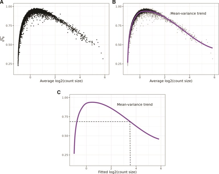
An important task in the analysis of spatially resolved transcriptomics (SRT) data is to identify spatially variable genes (SVGs), or genes that vary in a 2D space. Current approaches rank SVGs based on either $ P $-values or an effect size, such as the proportion of spatial variance. However, previous work in the analysis of RNA-sequencing data identified a technical bias with log-transformation, violating the "mean-variance relationship" of gene counts, where highly expressed genes are more likely to have a higher variance in counts but lower variance after log-transformation. Here, we demonstrate the mean-variance relationship in SRT data. Furthermore, we propose spoon, a statistical framework using empirical Bayes techniques to remove this bias, leading to more accurate prioritization of SVGs. We demonstrate the performance of spoon in both simulated and real SRT data. A software implementation of our method is available at https://bioconductor.org/packages/spoon.

Keywords: Gaussian process regression; empirical Bayes; mean–variance bias; spatial transcriptomics; spatially variable gene.

Fig. 1.

Calculating precision weights for individual observations. These data are from Invasive Ductal Carcinoma breast tissue analyzed with 10x Genomics Visium (10x Genomics 2022), hereafter referred to as “Ductal Breast.” A)–C) The square root of the residual standard deviations estimated using nearest neighbor Gaussian processes [ defined in (3)] are plotted against average logcount (). B) Same as A, except a spline curve is fitted to the data to estimate the gene-wise mean–variance relationship. C) Using the fitted spline curve, each predicted count value () is mapped to its corresponding square root standard deviation value using .

Fig. 2.

Mean–variance relationship exists in spatially resolved transcriptomics. Using data from different human tissues, in order from top to bottom: DLPFC (Maynard et al. 2021), Ductal Breast cancer (10x Genomics 2022), HPC (Thompson et al. 2024), LC (Weber et al. 2023a), and Ovarian cancer (Denisenko et al. 2024), we quantified the mean–variance relationship. Each point is a gene colored by the likelihood ratio statistic for a test that compares the fitted model against a classical linear model for the spatial component of variance using a NNGP (Weber et al. 2023b). The likelihood ratio statistics (LR Stat) are scaled by the maximum likelihood ratio statistic for each dataset in order to have more uniform visualization. The x-axis is mean logcounts and the y-axes represent different components of variance, in order from left to right: A) total variance , B) spatial variance , C) nonspatial variance , and D) proportion of spatial variance .

Fig. 3.

Mean-rank relationship exists in spatial transcriptomics data. Using three datasets, in order from top to bottom [DLPFC (Maynard et al. 2021), Ovarian cancer (10x Genomics 2022), and Lobular Breast cancer (10x Genomics 2020)], we quantified the mean-rank relationship. The genes were binned into deciles based on mean logcounts. Decile 1 contains the lowest mean expression values. The x-axis represents the rank. Within each decile, the density of the top 10% ranks is plotted as the signal in blue, while the density of the remaining ranks is plotted as the background in orange. Each subfigure shows the mean-rank relationship that persists after applying each method, from left to right: A), H), O) Moran’s I (Tsagris and Papadakis 2018), B), I), P) nnSVG (Weber et al. 2023b), C), J), Q) SPARK-X (Zhu et al. 2021), D), K), R) SpaGFT (Chang et al. 2024), E), L), S) SpatialDE2 (Kats et al. 2021), F), M), T) SMASH (Seal et al. 2023), and G), N), U) HEARTSVG (Yuan et al. 2024a).

Fig. 4.

Spoon removes the mean–variance relationship when detecting spatially variable genes. This dataset consists of 1,000 simulated genes across 968 spots using a lengthscale of 100. Separately for unweighted and weighted methods, the genes were binned into deciles based on mean logcounts. Decile 1 contains the lowest mean expression values. Ridge plots for the A) unweighted ranks and B) weighted ranks are shown. Within each decile (-axis), the density of the top 10% of ranks is plotted as the signal, while the density of the remaining ranks is plotted as the background. C) False discovery rate (FDR) as a function of Type I error (). As a function of FDR, we show the D) true negative rate (TNR) and E) true positive rate (TPR). The red represents weighted nnSVG and the blue represents unweighted nnSVG. These plots represent the average performance across five iterations of the same simulation, each with unique random seeds.

Fig. 5.

Spoon helps to detect SVGs associated with cancer that are lowly expressed. We used four datasets to evaluate the detection of cancer-related genes: ER+ Breast cancer (Wu et al. 2021a), Ovarian cancer (Denisenko et al. 2024), Lobular Breast cancer (10x Genomics 2020), and Ductal Breast cancer (10x Genomics 2022). A) Each bar contains the intersection of the set of genes of interest with genes within the set associated with cancer. For the first four rows, we defined low mean genes as those with means less than the 25th percentile in the dataset. Within the set of low mean genes, we found genes that were in the lowest 10% of ranks before weighting and then increased to the highest 10% of ranks after weighting. This is the set of genes of interest. The intersection in blue is the number of low mean and higher ranked genes that were found to be associated with the cancer of the dataset. For the last four rows, we defined low lengthscale genes as those with lengthscales between 40 and 90. Within the set of low lengthscale genes, we found genes that were ranked higher after weighting. This is the set of genes of interest. The intersection in pink shows the number of low lengthscale genes that were ranked higher and found to be associated with the cancer type of the dataset. B)–E) Within each dataset, the unweighted rank of each gene is plotted on the x-axis and the weighted rank on the y-axis. The genes related to cancer are labeled and colored by low lengthscale or low mean.

References

1. 10x Genomics. 2020. Human breast cancer: whole transcriptome analysis. https://www.10xgenomics.com/datasets/human-breast-cancer-whole-transcrip...
1. 10x Genomics. 2022. Human breast cancer: visium fresh frozen, whole transcriptome. https://www.10xgenomics.com/resources/datasets/human-breast-cancer-visiu...
1. Abrar MA, Kaykobad M, Rahman MS, Samee MAH. 2023. NoVaTeST: identifying genes with location-dependent noise variance in spatial transcriptomics data. Bioinformatics. 39:btad372. - PMC - PubMed
1. Ahlmann-Eltze C, Huber W. 2023. Comparison of transformations for single-cell RNA-seq data. Nat Methods. 20:665–672. - PMC - PubMed
1. Antolović V, Miermont A, Corrigan AM, Chubb JR. 2017. Generation of single-cell transcript variability by repression. Curr Biol. 27:1811–1817.e3. - PMC - PubMed